Press Release

Dissertation Example-MESHFREE METHODS FOR PDES ON SURFACES

Published

March 4, 2024

MESHFREE METHODS FOR PDES ON SURFACES

Andrew Michael Jones

A dissertation
submitted i n partial f ul llment
of the requirements for the degree of
Doctor of Philosophy in Computing
Boise State University

December 2022

BOISE STATE UNIVERSITY GRADUATE COLLEGE

DEFENSE COMMITTEE AND FINAL READING APPROVALS

of the dissertation submitted by

Andrew Michael Jones

Dissertation Title: Meshfree Methods for PDEs on Surfaces

Date of Final Oral Examination: 20 October 2022

The following individuals read and discussed the dissertation submitted by student Andrew Michael Jones, and they evaluated the students presentation and response to questions during the final oral examination. They found that the student passed the nal oral examination.

Grady B. Wright Ph.D. Chair, Supervisory Committee
Michal Kopera Ph.D. Member, Supervisory Committee
Min Long Ph.D. Member, Supervisory Committee
Peter A. Bosler Ph.D. Member, Supervisory Committee

The nal reading approval of the dissertation was granted by Grady B. Wright Ph.D., Chair of the Supervisory Committee. The dissertation was approved by the Graduate College.

DEDICATION

To my brothers: Daniel, David, and, Aaron. To my parents: Christina and Sinclair. To my partner and son: Monica and Rhydion.

ACKNOWLEDGMENT

Advisors and Collaborators

• Grady B. Wright
• Peter A. Bosler
• Varun Shankar
• Michal Kopera
• Paul A. Kuberry

Organizations: Boise State University, Sandia National Lab, University of Utah This work was partially supported the National Science Foundation Grant CCF 1717556. This work was also supported by the U.S. Department of Energy, O ce of Science, Advanced Scientific Computing Research (ASCR) Program and Biological and Environmental Research (BER) Program under a Scienti c Discovery through Advanced Computing (SciDAC 4) BER partnership pilot project.

This dissertation focuses on meshfree methods for solving surface partial di erential equations (PDEs). These PDEs arise in many areas of science and engineering where they are used to model phenomena ranging from atmospheric dynamics on earth to chemical signaling on cell membranes. Meshfree methods have been shown to be e ective for solving surface PDEs and are attractive alternatives to mesh-based methods such as nite di erences/elements since they do not require a mesh and can be used for surfaces represented only by a point cloud. The dissertation is subdivided into two papers and software.

In the rst paper, we examine the performance and accuracy of two popular mesh free methods for surface PDEs:generalized moving least squares (GMLS) and radial basis function- nite dierences (RBF-FD). While these methods are computationally e cient and can give high orders of accuracy for smooth problems, there are no published works that have systematically compared their bene ts and shortcomings. We perform such a comparison by examining their convergence rates for approximating the surface gradient, divergence, and Laplacian on the sphere and a torus as the resolution of the discretization increases. We investigate these convergence rates also as the various parameters of the methods are changed. We also compare the overall efficiencies of the methods in terms of accuracy per computation cost.

The second paper is focused on developing a novel meshfree geometric multilevel (MGM) method for solving linear systems associated with meshfree discretizations of elliptic PDEs on surfaces represented by point clouds. Multilevel (or multigrid) methods are e cient iterative methods for solving linear systems that arise in numerical PDEs. The key components for multilevel methods: grid coarsening, restriction/interpolation operators coarsening, and smoothing.

The first three components present challenges for meshfree methods since there are no grids or mesh structures,
only point clouds. To overcome these challenges, we develop a geometric point cloud coarsening method based on Poisson disk sampling, interpolation/ restriction opera tors based on RBF-FD, and apply Galerkin projections to coarsen the operator. We test MGM as a standalone solver and preconditioner for Krylov subspace methods on
various test problems using RBF-FD and GMLS discretizations, and numerically analyze convergence rates, scaling, and efficiency with increasing point cloud resolution. We finish with several application problems.

We conclude the dissertation with a description of two new software packages.

The first one is our MGM framework for solving elliptic surface PDEs. This package is built in Python and utilizes NumPy and SciPy for the data structures (arrays and sparse matrices), solvers (Krylov subspace methods, Sparse LU), and C++ for the smoothers and point cloud coarsening. The other package is the RBFToolkit which has a Python version and a C++ version. The latter uses the performance library Kokkos, which allows for the abstraction of parallelism and data management for shared memory computing architectures. The code utilizes OpenMP for CPU parallelism and can be extended to GPU architectures.

B PAPER 2:MGM:A MESHFREE GEOMETRIC MULTI LEVEL METHOD FOR LINEAR SYSTEMS ARISING FROM ELLIPTIC EQUATIONS ON POINT CLOUD SURFACES . . . . . . . . . . . . . . . . . . . . . . . .
B.1 Abstract . . . . . . . . . . . . . . . . . . . . . . . . . . . . . . . . . .
B.2 Introduction . . . . . . . . . . . . . . . . . . . . . . . . . . . . . . . .

B.2.1 Assumptions and notation . . . . . . . . . . . . . . . . . . . .
B.3 Localized mesh free discretizations . . . . . . . . . . . . . . . . . . . .

B.3.1 Tangent plane method . . . . . . . . . . . . . . . . . . . . . .
B.3.2 PHS-based RBF-FD with polynomials . . . . . . . . . . . . .
B.3.3 GFD. . . . . . . . . . . . . . . . . . . . . . . . . . . . . . . .

B.4 Multilevel transfer operators using R B Fs . . . . . . . . . . . . . . . .

B.5 Meshfree geometric multilevel(MGM)method . . . . . . . . . . . . .

B.5.1 Node coarsening. . . . . . . . . . . . . . . . . . . . . . . . . .
B.5.2 Coarse level operator . . . . . . . . . . . . . . . . . . . . . . .

B.5.3 Smoother and coarse level solver. . . . . . . . . . . . . . . . .

B.5.4 Modifications to the two-level cycle for the surface Poisson
problem . . . . . . . . . . . . . . . . . . . . . . . . . . . . . .

B.5.5 Multilevel extension . . . . . . . . . . . . . . . . . . . . . . .
B.5.6 Preconditioner for Krylov subspace methods . . . . . . . . . .

B.6 Numerical Results. . . . . . . . . . . . . . . . . . . . . . . . . . . . .

B.6.1 Stand alone solvervs. preconditioner. . . . . . . . . . . . . . .

B.6.2 Scaling with problemsize . . . . . . . . . . . . . . . . . . . .

B.6.3 Spectrum analysis. . . . . . . . . . . . . . . . . . . . . . . . .

B.6.4 Iteration vs.accuracy. . . . . . . . . . . . . . . . . . . . . . .

B.7 Applications . . . . . . . . . . . . . . . . . . . . . . . . . . . . . . . .
B.7.1 Surface harmonics. . . . . . . . . . . . . . . . . . . . . . . . .
B.7.2 Pattern formation. . . . . . . . . . . . . . . . . . . . . . . . .
B.7.3 Geodesic distance . . . . . . . . . . . . . . . . . . . . . . . . .
B.8 Concluding remarks. . . . . . . . . . . . . . . . . . . . . . . . . . . .

LIST OF FIGURES

1.1 Top row: Examples of domains where the di usion equation (1.2) can be solved analytically using separation of variables. Bottom row: examples of domains where separation of variables fails. . . . . . . . .

1.2 Illustrations of solutions to coupled reaction di usion PDEs Fitzhugh Nagumo spiral wave (left) on a unit sphere and Turing spots (right) on the Standford bunny. . . . . . . . . . . . . . . . . . . . . . . . . .

1.3 Illustrations of a surface discretized with a triangular tessellation (left) and with a point cloud (right). . . . . . . . . . . . . . . . . . . . . .

1.4 Illustration of RBF interpolation of 2D scattered data: (a) scattered data (b) radial basis functions (Gaussians), centered at data locations, and (c) interpolant of (a) . . . . . . . . . . . . . . . . . . . . . . . .

1.5 Structure (left) and unstructured (right) points on a square domain with a ve-point stencil. The red point is the stencil center, and the blue points represent the stencil neighbors. . . . . . . . . . . . . . . .

1.6 Illustration of two algorithms for determining nearest neighbors:-ball (left) and KNN search (right). The red point is the stencil center, and the blue points represent the stencil neighbors. . . . . . . . . . . . . .

1.7 Convergence plots for approximating the surface Laplacian on the torus (left) and sphere (right). . . . . . . . . . . . . . . . . . . . . . . . . .

1.8 Computational e ciency (Error vs. FLOPs) for approximating the surface Laplacian on the sphere: set-up (left) and run-time (right) costs. . . . . . . . . . . . . . . . . . . . . . . . . . . . . . . . . . . .

1.9 A schematic for a two-level V-cycle method for solving an elliptic PDE. 18 1.10 Illustration of the residual convergence results for = 7 RBF-FD discretizations of the sphere (left) and a cyclide (right) using MGM, PyAMG, preconditioners for GMRES and BiCGStab. . . . . . . . .

1.11 Left: Visualizations of the geodesic distance from the black dot marked on the Armadillo. The colormap transitions from white to yellow to indicate the increases in the distance. Right: Pattern formation on the
Stanford bunny. . . . . . . . . . . . . . . . . . . . . . . . . . . . . .

1.12 Github repositories for MGM and RBF Toolkit. . . . . . . . . . . . .

1.13 Comparison of residual convergence of various itertive methods for solving the screened Poisson equation on the sphere using a SE based discretization. . . . . . . . . . . . . . . . . . . . . . . . . . . . . . . .

A.1 Comparison of the two search algorithms used in this paper for deter mining a stencil. The nodes X are marked with solid black disks and all the stencil points are marked with solid blue disks, except for the stencil center, which is marked in red. . . . . . . . . . . . . . . . . . .

A.2 Illustration of a Monge patch parameterization for a local neighborhood of a regular surface M in 3D. (a) Entire surface (in gray) together with the tangent plane (in cyan) for a point xc where the Monge patch
is constructed (i.e., Txc M); red spheres mark a global point cloud X on the surface. (b) Close-up view of the Monge patch parameterization, together with the points from a stencil Xc (red spheres) formed from Xand the projection of the stencil to the tangent plane (blue spheres); the stencil center xc is at the origin of the axes for the xy-plane and is marked with a violet sphere. . . . . . . . . . . . . . . . . . . . . . .

A.3 Illustration of the tangent plane correction method. (a) Monge patch parameterization for a local neighborhood of a regular surface M (in gray) in 3D using a coarse approximation to the tangent plane (in yellow) at the center of the stencil xc and the re ned approximation to the tangent plane (in cyan). (b) Same as (a), but for the Monge patch with respect to the re ned tangent plane. The red spheres denote the points from the stencil and the blue spheres mark the projection of the stencil to the (a) coarse and (b) re ned tangent planes. The coarse andre ned approximations to the tangent and normal vectors are given as 1 c 2 , , and c, respectively, with tildes on these variables denoting the coarse approximation. . . . . . . . . . . . . . . . . . . . . . . . . . .

A.4 Convergence results for (a) surface gradient, (b) divergence, and (b) Laplacian on the sphere using icosahedral point sets. Errors are given in relative two-norms ( rst column) and max-norms (second column). Markers correspond to di erent : lled markers are GMLS and open markers are RBF-FD. Dash-dotted lines without markers correspond to 2nd, 4th, and 6th order convergence with 1 N. are the measured order of accuracy computed using the lines of best t to the last three reported errors. . . . . . . . . . . . . . . . . . . . . . . . . . . . . .

A.5 Same as Figure A.4, but for the cubed sphere points. . . . . . . . . .

A.6 Same as Figure A.4, but for the Poisson disk points on the sphere. . .

A.7 Same as Figure A.4, but for torus using Poisson disk points. . . . . .

A.8 Relative two-norm errors of the surface Laplacian approximations as the stencil radius parameter varies. Left gure shows errors for several di erent values of and a xed N = 130463. Right gure shows the convergence rates of the methods for di erent and a xed = 4. 68

B.1 Illustration of the tangent plane method for a 1D surface (curve). The solid black lines indicates the surface, the solid red circles mark the n =11 stencil nodes, the open blue circles mark the projected nodes, and the smarks the stencil center. (a) Direct projection of the stencil points according to (B.4). (b) Rotation and projection of the stencil points according to (B.6). . . . . . . . . . . . . . . . . . . . . . . . .

B.2 Illustration of the WSE algorithm for generating a coarse level set XH of NH = Nh 4 points from a ne level set Xh of Nh points. Here Nh = 14561 & NH = 3640 for the cyclide (a) and Nh = 14634 & NH =3658 for the Stanford Bunny (b) . . . . . . . . . . . . . . . . .

B.2.1 Assumptions and notation . . . . . . . . . . . . . . . . . . . .

B.3 Localized meshfree discretizations . . . . . . . . . . . . . . . . . . . .

B.3.1 Tangent plane method . . . . . . . . . . . . . . . . . . . . . .

B.3.2 PHS-based RBF-FD with polynomials . . . . . . . . . . . . .

B.3.3 GFD. . . . . . . . . . . . . . . . . . . . . . . . . . . . . . . .

B.4 Multilevel transfer operators using RBFs . . . . . . . . . . . . . . . .

B.5 Meshfree geometric multilevel(MGM)method . . . . . . . . . . . . .

B.5.1 Node coarsening. . . . . . . . . . . . . . . . . . . . . . . . . .

B.5.2 Coarse level operator . . . . . . . . . . . . . . . . . . . . . . .
B.5.3 Smoother and coarse level solver. . . . . . . . . . . . . . . . .

B.5.4 Modifications to the two-level cycle for the surface Poisson problem . . . . . . . . . . . . . . . . . . . . . . . . . . . . . .

B.5.5 Multilevel extension . . . . . . . . . . . . . . . . . . . . . . .

B.5.6 Preconditioner for Krylov sub space methods . . . . . . . . . .

B.6 Numerical Results. . . . . . . . . . . . . . . . . . . . . . . . . . . . .
B.6.1 Standalone solver vs. preconditioner. . . . . . . . . . . . . . .

B.6.2 Scaling with problem size . . . . . . . . . . . . . . . . . . . .
B.6.3 Spectrum analysis. . . . . . . . . . . . . . . . . . . . . . . . .
B.6.4 Iteration vs. accuracy. . . . . . . . . . . . . . . . . . . . . . .

B.7 Applications . . . . . . . . . . . . . . . . . . . . . . . . . . . . . . . .

B.7.1 Surface harmonics. . . . . . . . . . . . . . . . . . . . . . . . .
B.7.2 Pattern formation. . . . . . . . . . . . . . . . . . . . . . . . .
B.7.3 Geodesic distance . . . . . . . . . . . . . . . . . . . . . . . . .
B.8 Concluding remarks. . . . . . . . . . . . . . . . . . . . . . . . . . . .

LIST OF FIGURES

1.1 Top row: Examples of domains where the diffusion equation (1.2) can be solved analytically using separation of variables. Bottom row: examples of domains where separation of variables fails. . . . . . . . .

1.2 Illustrations of solutions to coupled reaction diffusion PDEs Fitzhugh Nagumo spiral wave (left) on a unit sphere and Turing spots (right) on the Stand ford bunny. . . . . . . . . . . . . . . . . . . . . . . . . .

1.3 Illustrations of a surface discretized with a triangular tessellation (left) and with a point cloud (right). . . . . . . . . . . . . . . . . . . . . .

1.7 Convergence plots for approximating the surface Laplacian on the torus (left) and sphere (right). . . . . . . . . . . . . . . . . . . . . . . . . .

1.9 A schematic for a two-level V-cycle method for solving an elliptic PDE. 18

1.10 Illustration of the residual convergence results for = 7 RBF-FD discretizations of the sphere (left) and a cyclide (right) using MGM, PyAMG, preconditioners for GMRES and BiCGStab. . . . . . . . .

1.11 Left: Visualizations of the geodesic distance from the black dot marked on the Armadillo. The colormap transitions from white to yellow to indicate the increases in the distance. Right: Pattern formation on the Stanford bunny. . . . . . . . . . . . . . . . . . . . . . . . . . . . . .

1.12 Github repositories for MGM and RBF Toolkit. . . . . . . . . . . . .

A.2 Illustration of a Monge patch parameterization for a local neighborhood of a regular surface M in 3D. (a) Entire surface (in gray) together with the tangent plane (in cyan) for a point xc where the Monge patch is constructed (i.e., Txc M); red spheres mark a global point cloud X on the surface. (b) Close-up view of the Monge patch parameterization, together with the points from a stencil Xc (red spheres) formed from Xand the projection of the stencil to the tangent plane (blue spheres); the stencil center xc is at the origin of the axes for the xy-plane and is marked with a violet sphere. . . . . . . . . . . . . . . . . . . . . . .

A.3 Illustration of the tangent plane correction method. (a) Monge patch parameterization for a local neighborhood of a regular surface M (ingray) in 3D using a coarse approximation to the tangent plane (in yellow) at the center of the stencil xc and the re ned approximation to the tangent plane (in cyan). (b) Same as (a), but for the Monge patch
with respect to the re ned tangent plane. The red spheres denote the points from the stencil and the blue spheres mark the projection of the stencil to the (a) coarse and (b) re ned tangent planes. The coarse and refined approximations to the tangent and normal vectors are given as 1 c 2 , c , and c, respectively, with tildes on these variables denoting the coarse approximation. . . . . . . . . . . . . . . . . . . . . . . . . . .

A.5 Same as Figure A.4, but for the cubed sphere points. . . . . . . . . .
A.6 Same as Figure A.4, but for the Poisson disk points on the sphere. . .
A.7 Same as Figure A.4, but for torus using Poisson disk points. . . . . .

B.1 Illustration of the tangent plane method for a 1D surface (curve). The solid black lines indicates the surface, the solid red circles mark the n =11 stencil nodes, the open blue circles mark the projected nodes, and the s marks the stencil center. (a) Direct projection of the stencil points according to (B.4). (b) Rotation and projection of the stencil points according to (B.6). . . . . . . . . . . . . . . . . . . . . . . . .

B.3 Convergence results for MGM and PyAMG based solvers for RBF-FD discretizations of a shifted Poisson problem with random right hand side. The sphere results are for Nh = 2621442, while for the cyclide Nh =2097152. . . . . . . . . . . . . . . . . . . . . . . . . . . . . . . .

B.4 Same as Figure B.3, but for GFD discretizations of the shifted surface Poisson problem. . . . . . . . . . . . . . . . . . . . . . . . . . . . . .

B.5 Wall-clock time (in seconds) for PyAMG GMRES and MGM GMRES to converge to a relative residual of 10 12 problem size (Nn) increases for RBF-FD (solid line) and GFD (dashed line) discretizations. The black dotted line marks linear scaling, O(Nh), for reference. . . . . . .

B.6 The spectra of the preconditioned matrix for shifted Poisson problem discretized with RBF-FD. . . . . . . . . . . . . . . . . . . . . . . . .

B.7 Relative residuals (left) and relative 2-norm errors (right) for solving a Poisson problem on the sphere with MGM GMRES. Solid lines cor respond to RBF-FD discretizations, while dashed lines correspond to GFD. . . . . . . . . . . . . . . . . . . . . . . . . . . . . . . . . . . .

B.8 Point clouds for the surfaces considered in the applications: Chinese Guardian Lion (N h = 436605), Stanford Bunny (N h = 291804), and Armadillo (N h = 872773). . . . . . . . . . . . . . . . . . . . . . . . .

B.9 Left: pseudocolor map of the rst 10 non-zero surface harmonics of the Chinese Guardian Lion model. . . . . . . . . . . . . . . . . . . . . . .

B.10 Left: pseudocolor map of the u variable in the numerical solution of (B.20) on the Stanford Bunny model; the colors transition from white to yellow to red to black, with white corresponding to u = 0 and black
to u = 1. Right: iteration count of MGM GMRES for solving the linear systems associated with u and v variables at each time-step in the semi-implicit scheme for (B.20). . . . . . . . . . . . . . . . . . . .

B.11 Left: pseudocolor map of the approximate geodesic distance from the solid circle on the chest of the Armadillo model (viewed from the front and backside) computed with the heat method. Solid black lines mark
the contours of the distance field and the colors transition from white to yellow to red with increasing distance from the solid circle. Right: iteration count of GMRES preconditioned with MGM for solving the linear systems associated with the heat method. . . . . . . . . . . . .

CHAPTER 1:

INTRODUCTION

1.1 Overview

This dissertation is comprised of two papers:

PI.

A. M. Jones, G. B. Wright, P. A. Bosler, P. A. Kuberry. A comparison of generalized moving least squares and radial basis function nite di erence methods for approximating surface derivatives. Submitted (2022)

PII.

G. B. Wright, A. M Jones, and V. Shankar. A meshfree geometric multilevel method for systems arising from elliptic equations on point cloud surfaces. SIAM Journal on Scienti c Computing. Accepted (2022) and two software packages:

SI.

A. M. Jones, MGM: Meshfree Geometric Multilevel Solver and Preconditioner. https://github.com/AndrewJ3/MGM

SII.

A. M. Jones, RBFToolkit: Radial basis function Toolkit. https://github.com/AndrewJ3/rbftoolkit PI is reproduced in Appendix A and the author contributions to this paper are described in Chapter 2. Similarly, PII is reproduced in Appendix B, with author contributions given in Chapter 3. Chapter 4 gives an overview of SI and SII. Finally,

Chapter 5 gives some concluding remarks on the work. The remainder of this chapter includes relevant background material on the topics of the thesis, overview of the contributions made, and some future work. References for Chapter 1 are given at the end of the chapter, while references for the PI and PII are included with the papers.

1.2 Mathematical modeling

Mathematical models provide a framework for predicting and understanding processes and phenomena in various elds ranging from the natural and social sciences to engineering. The prototypical example comes from classical mechanics formulated by Newton and others in the 17th century. If we have a projectile of mass m subjected to gravitational and linear drag forces Fg = mg and FD = ku(t), respectively and the velocity u(t) is changing over time t, then according to Newtons second law, we can sum the forces acting on the projectile to obtain a relation for the acceleration of the entire projectile. This gives the following system of ordinary differential equations (ODE) to solve for the velocity:

m = du(t)bydt = ku(t)+mg
(1.1)

For a given initial velocity u(0) = u0, this system of ODEs is linear and straight forward to solve analytically. Unfortunately, this is an exceptional situation. It is much more common that mathematical models for real-world applications can never be solved analytically. This can occur because of nonlinear relationships involving the unknowns, the unknowns also depending on space as well as time, and/or the spatial domains being geometrically complex.

Mathematical models for phenomena that depend on multiple variables, such as two or more spatial variables and/or time, typically lead to partial di erential equations (PDEs). A simple example is the di usion equation, which describes how some quantity di uses over time through a domain . In three dimensions, the PDE takes the form

(1.2)

where = xx + yy + zz is the Laplacian operator and > 0 is the diffusion coefficient, which depends on the medium of . To complete the model, we must also specify the initial conditions, and if has boundaries, then we must specify how the quantity behaves at the boundaries (commonly called boundary conditions). The diffusion equation (1.2), and other related linear PDEs like the Poisson and wave equations, can be solved with analytical methods like separation of variables or Fourier transforms, only for a very limited number of domains; we illustrate some of these simpler domains in the top row of Figure 1.1. However, even in these cases, the solutions depend on infinite sources and/or integrals that can not be computed analytically. If the domains have any geometric complexity, as illustrated in the bottom row of Figure 1.1. Then these analytical methods fail. In these cases, we are instead forced to solve these models approximately using numerical methods. This thesis focuses on numerical methods for mathematical models on geometrically complex domains, in particular, on PDEs posed on two-dimensional surfaces embedded in three dimensional space, such as the last three surfaces in Figure 1.1.

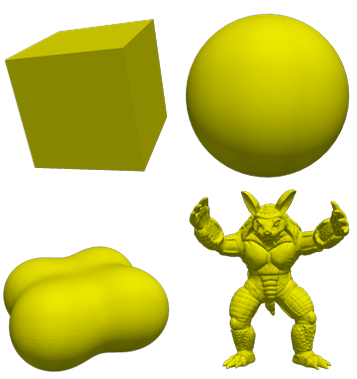
Figure 1.1: Top row: Examples of domains where the diusion equation (1.2) can be solved analytically using separation of variables. Bottom row: examples of domains where separation of variables fails.

1.3 Surface partial differential equations

Surface PDEs arise across many branches of science and engineering, for example, in atmospheric ows [63], bulk surface biomechanics [32], and computer graphics for texture generation [58]. An additional application is to activator and inhibitor systems modeled by surface reaction-di usion systems; some examples are shown in Figure 1.2. For our purposes, we focus primarily on PDEs like the diffusion and Poisson equations that are posed on smooth two-dimensional closed surfaces M R3.

Surface Di usion Equation: ut – Mu=f (1.3)
Screened Surface Poisson Equation: (a-m)u = f (1.4)

Here M is the surface Laplacian (or Laplace-Beltrami operator) on M, and is a parameter. The screened Poisson equation is equivalent to the non-homogenous Helmholtz equation with imaginary wave number. When = 0, the surface Poisson equation is recovered. For the remainder of the section, we discuss the historical development of surface PDEs and the mesh-based methods commonly used for solving and discretization (SE, FE, FV, FD). Lastly, we discuss the bene ts of meshfree methods for surface PDEs.

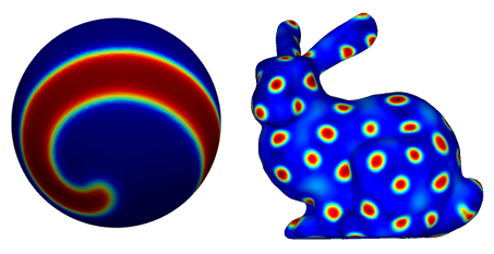
Figure 1.2: Illustrations of solutions to coupled reaction di usion PDEs Fitzhugh Nagumo spiral wave (left) on a unit sphere and Turing spots (right) on the Standford bunny.

Early numerical studies of surface PDEs were mainly restricted to the sphere and applied to problems in numerical weather prediction (NWP) [12, 51, 62, 43].

These early studies mainly utilized nite di erence and spectral methods, but in the 1980s and onward, additional methods were introduced based on nite volume methods (FV) [44, 64] and spectral/ nite element methods (FE/SE) [33, 54, 21]. Concurrently, solving PDEs on general surfaces was examined in the 1980s by [13] using surface FE (SFE) methods, and as interest in these PDEs grew, techniques were developed such as embedded nite element (EFE) [8, 35], and closest point (CP) [31] methods.

Development of meshfree methods for surface PDEs began in the early 2010s using global RBF methods [38, 19]; and development of localized versions of these methods soon followed, including radial basis function nite di erences (RBF FD) method [1, 28, 45, 39, 46, 61], generalized nite di erence (GFD) methods [52], and generalized moving least squares (GMLS) [29, 56, 23].

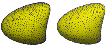
Figure 1.3: Illustrations of a surface discretized with a triangular tessellation (left) and with a point cloud (right).

In contrast with FE-based methods, which use tessellation of triangular or quadrilateral elements like SFE, and also they do not extend into the embedding space like EFE, meshfree techniques only require nodal points of mesh or simply a point cloud as illustrated by Figure 1.3. This allows for more algorithmic exibility. Meshfree

methods can also proce high order accurate approximationsfor smooth problems. This dissertation focuses on RBF-FD and GFD/GMLS methods for solving surface PDEs. Before outlining the motivations and contributions for this dissertation, we give a brief overview of the meshfree methods used in this work.

1.4 Global meshfree interpolation and approximation

1.4.1 Radial basis functions

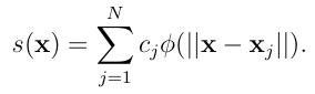
RBFs were originally developed in the 1970s for scattered data interpolation problems arising in cartography [24] and have subsequently been used in many applications, including for numerically solving PDEs starting in 1990 [26]. The RBF interpolation process is illustrated in Figure 1.4. This gure shows a reconstruction of data collected at scattered nodes using Gaussian RBFs. Starting with scattered data, the RBF method produces an interpolant of this data using a linear combination of rotations of a single radial kernel (e.g. the Gaussian) centered at each of the data sites. For xxj Rd, a general radial kernel centered at xj is de ned as (xxj) := ( x xj )where is the standard Euclidean norm and is a scalar function. Given a set of N points X = xk N k=1 Rd, the basic RBF interpolant to a function f sampled at X takes the form,

(1.5)

where the coe cients cj are determined by the interpolation conditions,

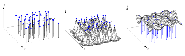
Figure1.4: Illustration of RBF interpolation of 2D scattered data: (a) scattered data (b) radial basis functions (Gaussians), centeredat data locations,and(c) interpolant of(a) .

Nsumofj=1 cj ( xi xj )=f(xi) i=1 N (1.6)

These conditions can be written as the following

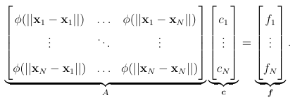
(1.7)

Some commonly used RBFs are the Gaussian, (r)=exp( (r)2),multi quadric, (r)= 1+(r)2,and poly harmonic splines(PHS), (r)=r2+1 and r 2 log r,where
R+is the shape parameter and Z+is the smoothness parameter. In this dissertation,we use PHS,which are advantageous because they do not require shape parameters. Choosing suitable shape parameters often require s expensive optimization algorithms [15], andthe interpolation matrix can be come extremely ill-conditioned
for small shape parameters,prompting the use of so-called stable algorithms[18]. When using PHS,one of ten appends on low degree polynomials to(1.4.1)to guarantee the well-posedness of the interpolation problem. However, more importantly, this has the added benefit of improving approximation convergence rates and allows
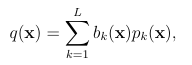
for polynomial reproduction [18]. The new form of the interpolant is as follows:

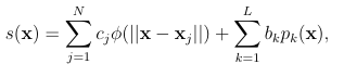
(1.8)

where pk L k=1 are a basis for d-variate polynomials of degree and L is the dimension of this space. To account for the new L coefficients, bk, the interpolant is subject to the following moment conditions [60, 45]:

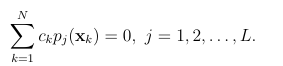
One issue with global RBF interpolation methods is that the linear system (1.7) is dense and not well suited for iterative methods. Direct methods require O(N3) computational cost, which becomes prohibitive for large N. To x this issue, we can use localized, stencil-based approximations as discussed in Section 1.5.

1.4.2 Polynomial moving least squares (MLS)

The development of MLS methods are mainly based on work done in the 1960s using moving averages for approximating irregular multivariate data in geophysics [48, 3]. Work involving such data had similar applications as RBF methods, such as meteorology and geography. MLS was re ned from early 1980s [27], with extensions to approximating PDEs in the 1990s [7] and the 2000s [30]. A MLS approximant to data f1 f2
fN sampled at X takes the form

(1.9)

where pk L k are again a basis for d-variate polynomials of degree . The coefficients of the approximant are determined from the following weighted least squares problem:

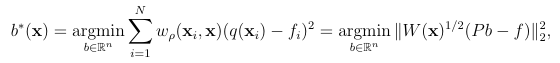
(1.10)

where W = diag(w(xi x)) and w is a non-negative kernel. Note that the coefficients depend on x because of the weight kernel. This is the origin of the name moving for MLS methods. Some examples of weighting kernels are given as follows,

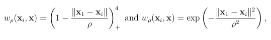
(1.11)

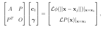
where is the support radius and ()+ is the positive oor operator. These weighting kernels will be reintroduced in later chapters when we discuss the GMLS methods. We can pose (B.12) as following (weighted) linear system

PTW(x)Pb =PTW(x)f, (1.12)

which are the normal equations to the weighted least squares problem. Provided that P has full rank and W(x) has strictly positive entries on its diagonal (1.12) has a unique solution. Note that this system must be solved for each evaluation point x, making MLS computationally expensive.

1.5 Localized meshfree methods

Localized meshfree methods were developed to reduce the high computational cost associated with global methods like RBFs. These methods use local interpolants/approximants over small stencils of points chosen from the global point set to approximate derivatives, similar to finite difference methods.

1.5.1 Stencils and nearest neighbor searches

A stencil is a collection of n << N points from a global point set X = xj N j=1 used for approximating a function f or some derivative of f at a point xc, called the stencil center. Some examples of stencils are provided in Figure 1.5 for structured and unstructured points X and n = 5. We denote a stencil with center xc = xk X as Xk = xj j k ,where k is the the index set containing the indices of the points in X contained in a stencil. The points are typically chosen as some collection of the nearest neighbors to xc. Figure A.1 illustrates two di erent techniques for determining these nearest neighbors: ball and K nearest neighbors (KNN), which can be implemented efficiently using a k-dimensional tree. Using the above notation, we can write a stencil-based approximation to a linear di erential operator L applied to a function u sampled at X as

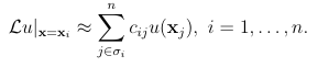
(1.13)

The weights cij depend on the locations, point spacings, stencil size, and approximation methods [18], which we discuss in the next section. Note that these weights can be assembled into a sparse N N stiffness matrix .

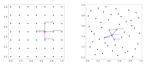
Figure 1.5: Structure (left) and unstructured (right) points on a square domain with a ve-point stencil. The red point is the stencil center, and the blue points represent the stencil neighbors.

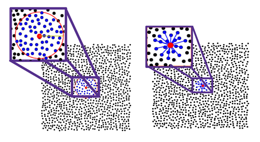
Figure 1.6: Illustration of two algorithms for determining nearest neigh
bors:-ball (left) and KNN search (right). The red point is the stencil
center, and the blue points represent the stencil neighbors.

1.5.2 RBF-FD

Suppose the rst stencil contains the points X1 = x1,….., xn . Then RBF-FD determines the weights c1j in (A.1) as the solution to the following system,

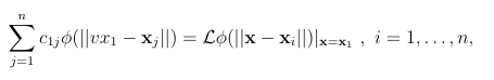
(1.14)

under the constraint that the weights c1j are exact for all polynomials of degree :

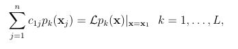
where pk L k=1, are again a basis for the set of polynomials of degree . As described in detail by [18], the weights satisfying (1.14) under the above constraints can be computed by solving the following linear system:

(1.15)

where A is given in (1.7) and Pjk = pk(xj), and is a Lagrange multiplier. The RBF FD weights for all the remaining stencils Xi i = 2,…..,N can be computed similarly using (1.15).

1.5.3 GMLS/GFD

The GMLS and GFD methods are very similar (and, in most cases, identical). The procedure for generating FD-type weights is similar to RBF-FD, except a local weighted polynomial least squares problem (B.12) is used. Using the notation from the previous section, the weights for the rst stencil X1 can be computed from the normal equations as follows:

c1 = W(x1)P(PTW(x1)P) 1Lpxc. (1.16)

In practice, one would use a QR factorization of W(x1)P for one to solve (1.16) in a numerically stable manner.

1.6 Node generation

Node or point cloud generation are initial or preprocessing stages of solving meshfree discretizations of PDEs on surfaces. Overall there are mesh-based and meshfree techniques for obtaining a point cloud. The mesh-based node generation can be straight-forward, since one simply requires extracting nodes from mesh elements, which must have good quality. A wide range of open source mesh generation packages are available such as Meshlab [37] or Gmsh [20]. Using mesh-based node generation can be computationally expensive and wasteful since we do not require all element information (i.e. faces, edges). Meshfree node generation has been explored on general planar domains and surfaces [66, 17, 47, 49] using node repulsion algorithms and Poisson disk sampling.

1.7 Contributions of this dissertation

1.7.1 Contributions of PI

Motivation

Many multi physics problems require the computation of derivatives on two-dimensional surfaces embedded in R3. For example, simulating atmospheric ows with Eulerian or Lagrangian numerical methods requires approximating surface gradients, diver

gence, and Laplacians of various quantities like wind, pressure, and bathymetry on the sphere [59, 43, 63, 18, 9].Similar di erential operators must be approximated for much more complicated surfaces than the sphere in application such as glaciology [22] in surface chemistry [65], computer graphics [34], multiphase ows with surfac tants [14], sea-air hydrodynamics [4, 2] and bulk-surface biomechanics [13, 42]. In short, surface derivatives are of great importance across many areas of science and engineering, and e cient and accurate methods are required for approximating these quantities.

RBF-FD and GMLS have separately been developed for this task and have shown to be quite e ective since they can produce high orders of accuracy at low computational cost, and they do not require any gridding or meshing. While some studies have been published comparing these methods for approximating functions and derivatives in R2 and R3 [6]. No published studies compare these methods for approximating derivatives on surfaces. This study aims to ll this gap and builds on the technical report of Jones and Bosler [25].

Overview

We examine the performance and accuracy of the two methods for approximating the surface gradient, divergence, and Laplacian. The focus is on how the methods compare with each other when stencil sizes, polynomial degrees, di erential operators, and point clouds vary. We additionally show for the rst time the equivalence of the two local formulations of the surface derivatives, which are designated as the local coordinate method and tangent plane method . For the problems we tested, we found that RBF-FD and GMLS methods converge at nearly the same rates when using the same polynomial degree, and RBF-FD gives lower errors for the same degrees of freedom. This is illustrated in Figure 1.7 for the surface Laplacian on the torus and sphere. Additionally, when comparing the accuracy of the methods versus the computational cost, we found that RBF-FD performs better when set-up costs are neglected. When these are accounted for, GMLS is more competitive. This is illustrated for the Laplacian on the sphere in Figure 1.8.

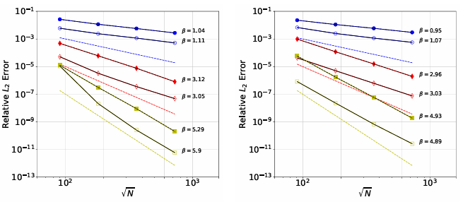
Figure 1.7: Convergence plots for approximating the surface Laplacian on the torus (left) and sphere (right).

1.7.2 Contributions of PII

Motivation

Meshfree methods for PDEs such as RBF-FD and GFD lead to large sparse linear systems of equations that need to be solved. To make these methods practical for large-scale problems, e ective iterative methods need to be developed for solving these systems. One class of iterative methods that are particularly effective at solving systems associated with standard FD discretizations are multilevel methods, such

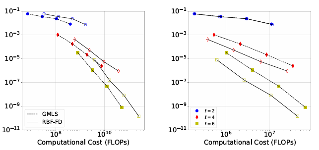
Figure 1.8: Computational e ciency (Error vs. FLOPs) for approximating the surface Laplacian on the sphere: set-up (left) and run-time (right) costs.

as geometric multigrid [10, 57]. However, since meshfree methods do not have an underlying grid structure, the extension of these methods to this setting is not apparent. There is also the need for solvers that can handle degenerate PDEs (surface Poisson equation) and high-order PDE discretizations. In this project, we focus on solving these challenges and develop a meshfree geometric multilevel (MGM) method for RBF-FD and GFD discretizations.

Overview

The components for any multilevel method are: a method for coarsening the points, a solver for the coarse level correction equations, restriction methods for the residuals, and an interpolation method for the corrections [10, 57]. The term smoother arises from the nature of a relaxation method (e.g. SOR, damped Jacobi, or Gauss-Seidel) to lter the high-frequency oscillations present in the error. This smoothing step is conducted on all grid levels until the coarsest grid is reached, where the coarse grid solution is computed. The next step is to prolongate (interpolate) the coarse solution to the original ne grid. This completes what is called the V-cycle iteration [10, 57], illustrated is shown in Figure 1.9.

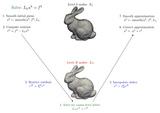
Figure 1.9: A schematic for a two-level V-cycle method for solving an elliptic PDE.

For a meshfree treatment of multilevel methods, we must have a hierarchy of increasingly coarser point clouds rather than grids. We address this challenge using a point cloud coarsening algorithm called weighted sample elimination [66]. The interpolation and restriction is done using RBF-FD with polyharmonic splines (PHS) plus constants. For the smoothing, we apply forward Gauss-Seidel, and a SparseLU for the coarse level solve. In the numerical tests, we examine the convergence with increasing polynomial and PHS degree using two meshfree discretizations: RBF-FD and GFD. MGM is used as preconditioner and a independent solver and compared with an algebraic multigrid software package PyAMG [36], some results for solving a screened Poisson problem 1.4 are displayed in Figure 1.10. We nish this paper with several application problems, computing geodesics distance and simulating pattern formation driven by nonlinear reaction-diffusion; see Figure 1.11 for an illustration.

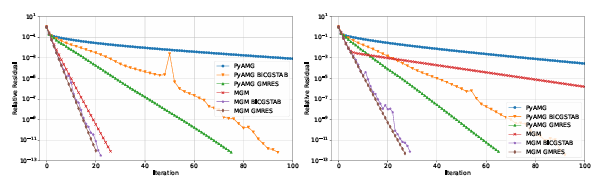
Figure 1.10: Illustration of the residual convergence results for = 7 RBF FD discretizations of the sphere (left) and a cyclide (right) using MGM, PyAMG, preconditioners for GMRES and BiCGStab.

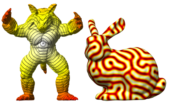
Figure 1.11: Left: Visualizations of the geodesic distance from the black dot marked on the Armadillo. The colormap transitions from white to yellow to indicate the increases in the distance. Right: Pattern formation on the Stanford bunny.

1.7.3 Contributions of PI and PII

We present two new software packages that were developed in conjunction with this thesis, MGM and RBFToolkit. MGM is a Python based meshfree multilevel solver for elliptic PDEs. The libraries NumPy, SciPy, PyAMG handle the data structures (n-dimensional arrays) and the numerical linear algebra (Krylov subspace methods, relaxation/smoothers methods), and Matplotlib provides the data visualization. The link to the code repository is https://github.com/AndrewJ3/MGM, the repository homepage is shown in Figure 1.12. RBFToolkit will be a refactor of the RBFKokkos C++code presented in [25]. This updated version will be written in Python and will include an improved C++ and Kokkos version. The repository can be found with the following link https://github.com/AndrewJ3/rbftoolkit, and the homepage is shown in Figure 1.12.

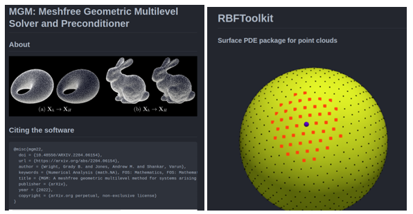
Figure 1.12: Github repositories for MGM and RBFToolkit.

1.8 Future work

Most studies of PDEs on the sphere focus on numerical weather prediction [51, 33, 43] and in the last century, numerous discretizations of the sphere have arisen. Early works in this area focus on latitude-longitude grids, which have failures due to sin gularities at the poles. This has prompted the examination of other spherical dis cretizations. Some of these other discretizations are the cubed sphere [44, 40] and icosahedral mesh, [5], which each have a variety of different arrangements. These grids are commonly used in FV/FE methods [63, 54]. Another family of grids is based on ideal spiral arrangements that can be derived from the Fibonacci sequence, referenced as Fibonacci grids [53]. Pseudo-random point distributions for the sphere have also been studied for point picking [31] and Monte Carlo methods [55]. Also, there is

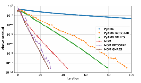
Figure 1.13: Comparison of residual convergence of various itertive methods for solving the screened Poisson equation on the sphere using a SE based discretization.

Poisson disk sampling which can produce quasi-uniform points e ciently [11]. An other study relevant to meshfree methods involves minimal energy [41] and maximum determinant [50] point clouds for the sphere, which have been used with RBF-FD for atmospheric ows [16]. Overall, no comprehensive study of PDEs on the sphere has been conducted for this wide range of point clouds and PDE discretizations. We address these areas of interest with some preliminary results using MGM to solve a SE discretization of the screened Poisson equation (1.4). We compare MGM with PyAMG and nd improved convergence rates when using MGM; these results are illustrated in Figure 1.13. Future work related to this dissertation, we will study the various sphere discretizations with MGM.

REFERENCES

[1] Alvarez, Diego, Gonzalez-Rodrguez, Pedro, and Kindelan, Manuel. 2021. A Local Radial Basis Function Method for the LaplaceBeltrami Operator. J. Sci. Comput., 86(3), 28.

[2] Asher, William E., Liang, Hanzhuang, Zappa, Christopher J., Loewen, Mark R., Mukto, Moniz A., Litchendorf, Trina M., and Jessup, Andrew T. 2012. Statistics of surface divergence and their relation to air-water gas transfer velocity. Journal of Geophysical Research: Oceans, 117(C5).

[3] Backus, George, and Gilbert, Freeman. 1968. The Resolving Power of Gross Earth Data. Geophysical Journal International, 16(2), 169205.

[4] Banerjee, Sanjoy, Lakehal, Djamel, and Fulgosi, Marco. 2004. Surface divergence models for scalar exchange between turbulent streams. International Journal of Multiphase Flow, 30(7), 963977. A Collection of Papers in Honor of Professor G. Yadigaroglu on the Occasion of his 65th Birthday.

[5] Baumgardner, John, and Frederickson, Paul O. 1985. Icosahedral Discretization of the Two-Sphere. SIAM Journal on Numerical Analysis, 22, 11071115.

[6] Bayona, Victor. 2019. Comparison of Moving Least Squares and RBF+Poly for Interpolation and Derivative Approximation. Journal of Scienti c Computing, 81(1), 486512.

[7] Belytschko, T., Lu, Y. Y., and Gu, L. 1994. Element-free Galerkin methods. International Journal for Numerical Methods in Engineering, 37(2), 229256.

[8] Bertalmo, M., Cheng, L., Osher, S., and Sapiro, G. 2001. Variational problems and partial di erential equations on implicit surfaces. J. Comput. Phys., 174, 759780.

[9] Bosler, P.A., Wang, L., Jablonowski, C., and Krasny, R. 2014. A Lagrangian particle/panel method for the barotropic vorticity equations on a rotating sphere. Fluid Dyn. Res., 46.

[10] Brandt, A., and Livne, O.E. 2011. Multigrid Techniques: 1984 Guide with Applications to Fluid Dynamics, Revised Edition. Classics in Applied Mathematics. Society for Industrial and Applied Mathematics.

[11] Bridson, Robert. 2007. Fast Poisson Disk Sampling in Arbitrary Dimensions.22 es.

[12] Charney, J. G., FjOrtoft, R., and Neumann, J. Von. 1950. Numerical Integration of the Barotropic Vorticity Equation. Tellus, 2(4), 237254.

[13] Dziuk, G. 1988. Finite elements for the Beltrami operator on arbitrary surfaces. In: Hildebrandt, S., and Leis, R. (eds), Partial Di erential Equations and Calculus of Variations. Lecture Notes in Mathematics, vol. 1357. Berlin: Springer.

[14] Erik Teigen, Knut, Song, Peng, Lowengrub, John, and Voigt, Axel. 2011. A diffuse-interface method for two-phase ows with soluble surfactants. Journal of Computational Physics, 230(2), 375393.

[15] Fasshauer, G., and Zhang, J. 2007. On choosing optimal shape parameters for RBF approximation. Numerical Algorithms, 45, 345368.

[16] Flyer, Natasha, and Wright, Grady B. 2009. A radial basis function method for the shallow water equations on a sphere. Proceedings of the Royal Society A: Mathematical, Physical and Engineering Sciences, 465(2106), 19491976.

[17] Fornberg, Bengt, and Flyer, Natasha. 2015a. Fast generation of 2-D node distributions for mesh-free PDE discretizations. Computers Mathematics with Applications, 69(7), 531544.

[18] Fornberg, Bengt, and Flyer, Natasha. 2015b. A Primer on Radial Basis Functions with Applications to the Geosciences. Philadelphia, PA, USA: Society forIndustrial and Applied Mathematics.

[19] Fuselier, Edward J., and Wright, Grady B. 2013. A High-Order Kernel Method for Di usion and Reaction-Di usion Equations on Surfaces. Journal of Scienti c Computing, 56(3), 535565.

[20] Geuzaine, Christophe, and Remacle, Jean-Francois. 2009. Gmsh: A 3-D niteelement mesh generator with built-in pre- and post-processing facilities. International Journal for Numerical Methods in Engineering, 79(11), 13091331.

[21] Giraldo, Francis X. 1997. LagrangeGalerkin Methods on Spherical Geodesic Grids. Journal of Computational Physics, 136(1), 197213.

[22] Gowan, Evan J., Zhang, Xu, Khosravi, Sara, Rovere, Alessio, Stocchi, Paolo, Hughes, Anna L. C., Gyllencreutz, Richard, Mangerud, Jan, Svendsen, John-Inge, and Lohmann, Gerrit. 2021. A new global ice sheet reconstruction for the past 80000 years. Nature Communications, 12(1), 1199.

[23] Gross, B.J., Trask, N., Kuberry, P., and Atzberger, P.J. 2020. Meshfree methods on manifolds for hydrodynamic ows on curved surfaces: A Generalized Moving Least-Squares (GMLS) approach. Journal of Computational Physics, 409, 109340.

[24] Hardy, Rolland L. 1971. Multiquadric equations of topography and other irregular surfaces. Journal of Geophysical Research (1896-1977), 76(8), 19051915.

[25] Jones, Andrew M., and Bosler, Peter A. Radial Basis Functions in the Tan gent Plane: Meshfree Approximation Methods for the Sphere. Computer Science Research Institute Summer Proceedings 2020, 5767.

[26] Kansa, E.J. 1990. Multiquadrics-A scattered data approximation scheme with applications to computational uid-dynamics-II solutions to parabolic, hyperbolic and elliptic partial di erential equations. Computers and Mathematics with Applications.

[27] Lancaster, P., and Salkanskas, K. 1980. Surface Generated by Moving Least Squares Methods. American Mathematical Society.

[28] Lehto, E, Shankar, V, and Wright, G. B. 2017. A radial basis function (RBF) compact nite di erence (FD) scheme for reaction-diffusion equations on surfaces. SIAM J. Sci. Comput., 39, A219A2151.

[29] Liang, Jian, and Zhao, Hongkai. 2013. Solving Partial Di erential Equations on Point Clouds. SIAM J. Sci. Comput., 35(3), A1461A1486.

[30] Liu, Gui-Rong. 2009. Meshfree methods: moving beyond the nite element method. Taylor & Francis.

[31] MacDonald, C. B., and Ruuth, S. J. 2009. The implicit closest point method for the numerical solution of partial differential equations on surfaces. SIAM J. Sci. Comput., 31, 43304350.

[32] Madzvamuse, Anotida, Chung, Andy H. W., and Venkataraman, Chandrasekhar. 2015. Stability analysis and simulations of coupled bulk-surface reaction di usion systems. Proceedings of the Royal Society A: Mathematical, Physical and Engineering Sciences, 471(2175), 20140546.

[33] Mailhot, J., and Benoit, R. 1982. A Finite-Element Model of the Atmospheric Boundary Layer Suitable for Use with Numerical Weather Prediction Models. Journal of Atmospheric Sciences, 39(10), 2249 2266.

[34] Mikkelsen, Morten S. 2020. Surface GradientBased Bump Mapping Framework. Journal of Computer Graphics Techniques (JCGT), 9(4), 6091.

[35] Olshanskii, Maxim A., Reusken, Arnold, and Grande, Jorg. 2009. A Finite Element Method for Elliptic Equations on Surfaces. SIAM Journal on Numerical Analysis, 47(5), 33393358.

[36] Olson, L. N., and Schroder, J. B. 2018. PyAMG: Algebraic Multigrid Solvers in Python v4.0. Release 4.0.

[37] Paolo Cignoni, Alessandro Muntoni, Guido Ranzuglia Marco Callieri. MeshLab.

[38] Piret, Cecile. 2012. The orthogonal gradients method: A radial basis functions method for solving partial di erential equations on arbitrary surfaces. J. Comput.Phys., 231, 46624675.

[39] Piret, Cecile, and Dunn, Jarrett. 2016. Fast RBF OGr for solving PDEs on arbitrary surfaces. AIP Conference Proceedings, 1776(1), 070005.

[40] Putman, William M., and Lin, Shian-Jiann. 2007. Finite-volume transport on various cubed-sphere grids. Journal of Computational Physics, 227(1), 5578.

[41] Rakhmanov, Evguenii A, Sa , Edward B, and Zhou, YM1306011. 1994. Minimal discrete energy on the sphere. Mathematical Research Letters, 1(6), 647662.

[42] Ratz, Andreas, and Roger, Matthias. 2014. Symmetry breaking in a bulk-surface reaction-di usion model for signaling networks. Nonlinearity, 27(8), 1805.

[43] Richardson, Lewis Fry, and Lynch, Peter. 2007. Weather Prediction by Numerical Process. 2 edn. Cambridge Mathematical Library. Cambridge University Press.

[44] Ronchi, C., Iacono, R., Struglia, M.V., Rossi, A., Truini, C., Paolucci, P.S., and Pratesi, S. 1997.- The cubed sphere: A new method for solving PDEs on the sphere. applications to climate modeling and planetary circulation problems. Pages 3138 of: Schiano, P., Ecer, A., Periaux, J., and Satofuka, N. (eds), Parallel Computational Fluid Dynamics 1996. Amsterdam: North-Holland.

[45] Shankar, Varun, Wright, Grady B., Kirby, Robert M., and Fogelson, Aaron L.2014. A Radial Basis Function (RBF)-Finite Di erence (FD) Method for Di usion and Reaction-Di usion Equations on Surfaces. J. Sci. Comput., 63(3), 745 768.

[46] Shankar, Varun, Narayan, Akil, and Kirby, Robert M. 2018a. RBF-LOI: Augmenting Radial Basis Functions (RBFs) with Least Orthogonal Interpolation (LOI) for solving PDEs on surfaces. J. Comput. Phys., 373, 722735.

[47] Shankar, Varun, Kirby, Robert M., and Fogelson, Aaron L. 2018b. Robust Node Generation for Mesh-free Discretizations on Irregular Domains and Surfaces. SIAM Journal on Scienti c Computing, 40(4), A2584A2608.

[48] Shepard, Donald. 1968. A Two-Dimensional Interpolation Function for Irregularly-Spaced Data. Page 517524 of: Proceedings of the 1968 23rd ACM National Conference. ACM 68. New York, NY, USA: Association for Computing Machinery.

[49] Slak, Jure, and Kosec, Gregor. 2019. On generation of node distributions for meshless PDE discretizations. SIAM journal on scienti c computing, 41(5), A3202A3229.

[50] Sloan, Ian H, and Womersley, Robert S. 2004. Extremal systems of points and numerical integration on the sphere. Advances in Computational Mathematics, 21(1), 107125.

[51] Spinelli, R. A. 1965. Poisson Equation on a Sphere. Journal of the Society for Industrial and Applied Mathematics Series B Numerical Analysis, 2(3), 489 499.

[52] Suchde, Pratik, and Kuhnert, Jorg. 2019. A meshfree generalized nite difference method for surface PDEs. Comp. Math. Appl., 78(8), 27892805.

[53] Swinbank, Richard, and James Purser, R. 2006. Fibonacci grids: A novel approach to global modelling. Quarterly Journal of the Royal Meteorological Society, 132(619), 17691793.

[54] Taylor, Mark, Tribbia, Joseph, and Iskandarani, Mohamed. 1997. The Spectral Element Method for the Shallow Water Equations on the Sphere. Journal of Computational Physics, 130(1), 92108.

[55] Tichy, Robert F. 1990. Random points in the cube and on the sphere with applications to numerical analysis. Journal of Computational and Applied Mathematics, 31(1), 191197.

[56] Trask, Nathaniel, Patel, Ravi G, Atzberger, Paul J, and Gross, Ben J. 2020. GMLS-Nets: A Machine Learning Framework for Unstructured Data. In: AAAI Spring Symposium: MLPS.

[57] Trottenberg, Ulrich, Oosterlee, Cornelis W., and Schuller, Anton. 2001. Multi grid. Texts in Applied Mathematics. Bd., vol. 33. San Diego [u.a.]: Academic Press. With contributions by A. Brandt, P. Oswald and K. Stuben.

[58] Turk, Greg. 1991. Generating textures on arbitrary surfaces using reaction diffusion. Comput. Graph., 25(4), 289298.

[59] Vallis, Geo rey K. 2006. Atmospheric and Oceanic Fluid Dynamics: Fundamentals and Large-scale Circulation. Cambridge University Press.

[60] Wendland, Holger. 2004. Scattered Data Approximation. Cambridge Monographs on Applied and Computational Mathematics. Cambridge University Press.

[61] Wendland, Holger, and Kunemund, Jens. 2020. Solving partial di erential equations on (evolving) surfaces with radial basis functions. Advances in Computational Mathematics, 46, 64.

[62] White, P. W. 1971. Finite-Di erence Methods in Numerical Weather Prediction. Proceedings of the Royal Society of London. Series A, Mathematical and Physical Sciences, 323(1553), 285 292.

[63] Williamson, David L. 2007a. The Evolution of Dynamical Cores for Global Atmospheric Models. Journal of the Meteorological Society of Japan 85B, 241269.

[64] Williamson, David L. 2007b. The Evolution of Dynamical Cores for Global Atmospheric Models. J. Meteorol. Soc. Jpn., 85B, 241269.

[65] Yu, Xi, Wang, Zhiqiang, Jiang, Yugui, and Zhang, Xi. 2006. Surface Gradient Material: From Superhydrophobicity to Superhydrophilicity. Langmuir, 22(10), 44834486.

[66] Yuksel, Cem. 2015. Sample Elimination for Generating Poisson Disk Sample Sets. Computer Graphics Forum (Proceedings of EUROGRAPHICS 2015), 34(2), 25 32.

CHAPTER 2:

A COMPARISON OF GENERALIZED MOVING
LEAST SQUARES AND RADIAL BASIS
FUNCTION FINITE DIFFERENCE METHODS
FOR APPROXIMATING SURFACE
DERIVATIVES

A.1 Abstract

Approximating differential operators defined on two-dimensional surfaces is an important problem that arises in many areas of science and engineering. Over the past ten years, localized meshfree methods based on generalized moving least squares (GMLS) and radial basis function nite di erences (RBF-FD) have been shown to be e ective for this task as they can give high orders of accuracy at low computational cost, and they can be applied to surfaces defined only by point clouds. However, there have yet to be any studies that perform a direct comparison of these methods for approximating surface differential operators (SDOs). The purpose of this work is to ll that gap. We focus on RBF-FD methods based on polyharmonic spline (PHS) kernels and polynomials since they are most closely related to the GMLS method.

We give a detailed description of both methods, including the di erent ways that they formulate SDOs. One key nding we make here is that these formulations are equivalent when the tangent space to the surface is known exactly. We numerically examine the convergence rates of the methods for various parameter choices as the discretizations of the surfaces are re ned. We also compare their efficiency in terms of accuracy per computation cost.

A.2 Introduction

The problem of approximating differential operators defined on two dimensional surfaces embedded in R3 arises in many multiphysics models. For example, simulating atmospheric ows with Eulerian or Lagrangian numerical methods requires approximating the surface gradient, divergence, and Laplacian on the two-sphere [38, 42, 15, 8].
Similar surface differential operators (SDOs) must be approximated on more geometrically complex surfaces in models of ice sheet dynamics [17], biochemical signalingon cell membranes [23], morphogenesis [34], texture synthesis [25], and sea-air hydro dynamics [2].

Localized meshfree methods based on generalized moving least squares (GMLS) and radial basis function nite di erences (RBF-FD) have become increasingly popular over the last ten years for approximating SDOs and solving surface partial differential equations (PDEs) (see, for example, [24, 22, 36, 35, 18] for GMLS and [1, 21, 14,
31, 30, 32, 33, 29, 43, 19, 41] for RBF-FD methods). This is because they can provide high accuracy at low computational cost and can even be applied to surfaces defined by point clouds, without having to form a triangulation like surface finite element methods [12] or a level-set representation like embedded nite element methods [7]. While there is one study dedicated to comparing these methods for approximating functions and derivatives in R2 and R3 [3], there are no studies that compare the methods for approximating SDOs. The present work aims to ll this gap.

The RBF-FD methods referenced above use di erent approaches for approximating SDOs, while the GMLS methods essentially use the same approach. To keep the comparison to GMLS manageable, we will thus limit our focus to the RBF-FD method based on polyharmonic spline (PHS) kernels augmented with polynomials since they are most closely related to GMLS [3]. Additionally, these RBF-FD methods are becoming more and more prevalent as they can give high orders of accuracy that are controlled by the augmented polynomial degree [5] and they do not require choosing a shape parameter, which can be computationally intensive to do in an automated way. The RBF-FD methods referenced above also use distinct techniques for formulating the SDOs.

To again keep this comparison manageable, we limit our focus to the so-called tangent plane formulation, as it provides a more straight forward technique for incorporating polynomials in the PHS-based RBF-FD methods than [1, 21, 14, 31, 30, 32, 29, 41]. Additionally, the comparison in [33] of several RBF-FD methods for approximating the surface Laplacian (Laplace-Beltrami operator) revealed the tangent plane approach to be the most computationally efficient interms of accuracy per computational cost. The tangent plane method was first introduced by Demanet [11] for approximating the surface Laplacian using polynomial based approximations. Suchde & Kuhnert [35] generalized this method to other SDOs using polynomial weighted least squares to generate the stencil weights. Shaw [33] (see also [43]) was the rst to use this method for approximating the surface Laplacian with RBF-FD and Gunderman et. al. [19] independently developed the method for RBF-FD specialized to the surface gradient and divergence on the unit two-sphere.

The GMLS and RBF-FD methods are similar in that they use weighted combinations of function values over a local stencil of points to approximate SDOs. They also feature a parameter for controlling the degree of polynomial precision of the formulas. However, they also have several major di erences. First, GMLS is based on weighted least squares polynomial approximants, whereas the type of RBF-FD method considered here is based on PHS interpolants augmented with polynomials. Second, for GMLS one has to choose a weight kernel for the least squares problem, while one has to choose the order of the PHS kernel in the RBF-FD method. Third, GMLS uses local coordinates and approximations to metric terms to formulate the SDOs. The RBF-FD method examined in this study, on the other hand, is based on the tangent plane method, which does not explicitly include any metric terms. In this study, we compare GMLS and RBF-FD for approximating the surface gradient, divergence, and Laplacian operators on two topologically distinct surfaces, the unit two-sphere and the torus, which are representative of a broad range of application domains. We investigate their convergence rates as the sampling density of points on these surfaces increases for various parameter choices, including polynomial degree
and stencil sizes. In the case of the sphere, we also study the convergence rates of the methods for di erent point sets, including two popular ones used in applications: icosahedral and cubed sphere points. Finally, we investigate the efficiency of the methods in terms of their accuracy versus computational cost, both when including and excluding setup costs.

One key result we show analytically is that the local coordinate formulation of SDOs used in GMLS is identical to the formulation of the tangent plane method when the tangent space for the surface is known exactly for the given point cloud. Furthermore, our numerical results demonstrate that RBF-FD and GMLS give similar convergence rates for the same choice of polynomial degree , but overall RBF-FD results in lower errors. We also show that the often-reported super convergence of GMLS for the surface Laplacian only happens for highly structured, quasi-uniform point sets, and when the point sets are more general (but still possibly quasi-uniform), this convergence rate drops to the theoretical rate. Additionally, we find that the errors for RBF-FD can be further reduced with increasing stencil sizes, but that this does not generally hold for GMLS, and the errors can actually deteriorate. Finally, we find that when setup costs are included, GMLS has an advantage in terms of efficiency, but if these are neglected then RBF-FD is more efficient. The remainder of the paper is organized as follows. In Section A.3, we provide some background and notation on stencil-based approximations and on surface differential operators. We follow this with a detailed overview of the GMLS and RBF methods in Section A.4 and B.3.2, respectively. In Section A.6 we compare the two methods in terms of some of their theoretical properties and in Section B.6 we give an extensive numerical comparison of the methods. We end with some concluding remarks in Section A.8.

A.3 Background and notation

A.3.1 Stencils

The RBF-FD and GMLS methods both discretize SDOs by weighted combinations of function values over a local stencil of points. This makes them similar to traditional finite-difference methods, but the lack of a grid, a tuple indexing scheme, and inherent awareness of neighboring points requires that some di erent notation and concepts be introduced. In this section we review the stencil notation that will be used in the subsequent sections.
Let X = xi N i=1 be a global set of points (point cloud) contained in some domain.
A stencil of X is a subset of n N nodes of X that are close (see discussion below for what this means) to some point xc , which is called the stencil center. In this work, the stencil center is some point from X, so that xc = xi, for some
1 i N, and this point is always included in the stencil. We denote the subset of points making up the stencil with stencil center xi as Xi and allow the number of points in the stencil to vary with xi. To keep track of which points in Xi belong to X, we use index set notation and let i denote the set of indices of the 1 < ni N points from X that belong to Xi. Using this notation, we write the elements of the stencil as Xi = xj j i. We also use the convention that the indices are sorted by the distance the stencil points are from the stencil center xi, so that the rst element
of i is i. With the above notation, we can de ne a general stencil-based approximation method to a given (scalar) linear di erential operator L. Let u be a scalar-valued function de ned on that is smooth enough so that Lu is de ned for all x the approximation to Lu at any xi X is given as

(a.1)

The weights cij are determined by the method of approximation, which in this study will be either GMLS or RBF-FD. These weights can be assembled into a sparse N N sti ness matrix, similar to mesh-based methods. Vector linear differential operators (e.g., the gradient) can be similarly defined where (A.1) is used for each component and L is the scalar operator for that component. There are two main approaches used in the meshfree methods literature for determining the stencil points, one based on k-nearest neighbors (KNN) and one based on ball searches. These are illustrated in Figure A.1 for a scattered point set X in the plane. The approach that uses KNN is straightforward since it amounts to simply choosing the stencil Xi as the subset of ni points from X that are closest to xi. The approach that uses ball searches is a bit more involved, so we summarize it in Algorithm 1. Both methods attempt to select points such that the stencil satis es polynomial unisolvency conditions (see the discussion in Section A.4.1). In this work, we use the method in Algorithm 1 since

• it is better for producing stencils with symmetries when X is regular, which can

Algorithm 1: Procedure for determining the stencil points based on ball
searches.

1 Input: Point cloud X; stencil center xc; number initial stencil points n;
radius factor t 1;
2 Output: Indices c in X for the stencil center xc;
3 Find the n nearest neighbors in X to xc, using the Euclidean distance;
4 Compute the max distance hmax between xc and its n nearest neighbors;
5 Find the indices c of the points in X contained in the ball of radius th max centered at xc;

be beneficial for improving the accuracy of the approximations;

• it is more natural to use with the weighting kernel inherent to GMLS; and
• it produces stencils that are not biased in one direction when the spacing of the points in X are anisotropic.

To measure distance in the ball search, we use the standard Euclidean distance measured in R3 rather than distance on the surface since this is simple to compute for any surface. We also use a k-d tree to efficiently implement the method. Finally, the choice of parameters we use in Algorithm 1 are discussed in Section A.4.3.

A.3.2 Surface differential operators in local coordinates

Here we review some di erential geometry concepts that will be used in the subsequent sections. Much of this material can be found in a general book on this subject, e.g. [39, 28].

We as sume that M R3 isaregular, orientable surface so that it can be described by an atlas of local smooth charts [39]. Let TxM denote the tangent space to M at x M.Wecanexpress surface di erentiable operators in a neighborhood of x M

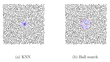
Figure A.1: Comparison of the two search algorithms used in this paper for determining a stencil. The nodes X are marked with solid black disks and all the stencil points are marked with solid blue disks, except for the stencil center, which is marked in red.

using the local chart

f =(xyf(xy)) (A.2)

where x, y are local coordinates for TxM, and f(xy) can be interpreted as a function over the xy-plane. This local parametric representation of M about x is called the Monge patch or Monge form [28] and is illustrated for a bumpy sphere surface in Figure B.1. Using this parameterization, the local metric tensor G about x for the surface is given as

(a.3)

Letting gij denote the (i j) entry of G1, the surface gradient operator locally about x is given as

M=( xf) g11 x+g12 y +( yf) g21 x+g22 y
(A.4)

However, this is the surface gradient with respect to the horizontal xy-plane (see Figure B.1 (b)), and subsequently needs to be rotated so that it is with respect to TxM in its original con guration. If 1 and 2 are orthonormal vectors that span TxM and is the unit outward normal to M at x, then the surface gradient in the correct orientation is given as

(a.5)

Using this result, the surface divergence of a smooth vector u TxM can be written
as

M u= g11 x+g12 y ( xf)TRTu+ g21 x+g22 y ( yf)TRTu
(A.6)

The surface Laplacian operator locally about x is given as

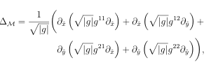
(a.7)

where g = det(G). This operator is invariant to rotations of the surface in R3, so

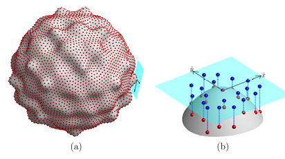
Figure A.2: Illustration of a Monge patch parameterization for a local neighborhood of a regular surface M in 3D. (a) Entire surface (in gray) together with the tangent plane (in cyan) for a point xc where the Monge patch is constructed (i.e., Txc M); red spheres mark a global point cloud X on the surface. (b) Close-up view of the Monge patch parameterization, together with the points from a stencil Xc (red spheres) formed from X and the projection of the stencil to the tangent plane (blue spheres); the stencil center xc is at the origin of the axes for the xy-plane and is marked with a violet sphere.

no subsequent modi cations of (A.7) are necessary.

A.4 GMLS using local coordinates

The formulation of GMLS on a manifold was introduced by Liang & Zhao [22] and further re ned by Trask, Kuberry, and collaborators [36, 18]. It uses local coordinates to approximate SDOs as de ned in (A.5) (A.7) and requires a method to also approximate the metric terms. Both approximations are computed for each xi X M using GMLS over a local stencil of points Xi X. Below we give a brief overview of the method assuming that the tangent/normal vectors for the surface are known for each xi X. We then discuss a method for approximating these that is used in the

Compadre Toolkit [20], which we use in the numerical experiments.

We present the GMLS method through the lens of derivatives of MLS approximants as we feel this makes the analog to RBF-FD clearer, it is also closer to the description from [22]. Other derivations of GMLS are based on weighted least squares approximants of general linear functionals given at some set of points, e.g. [40, 27, 37]. However, both techniques produce the same result in the end [27]. For a more thorough discussion of MLS approximants, see for example [13, ch. 22] and the references therein.

A.4.1 Approximating the metric terms

The metric terms are approximated from an MLS reconstruction of the Monge patch of M centered at each target point xi using a local stencil of ni points XiX. This procedure is illustrated in Figure B.1 and can be described as follows. First, the stencil Xi is expressed in the form of (A.2) (i.e., (xj yj fj), ji), where (xj yj) are the coordinates for the stencil points in Txi M, and fj = f(xj yj) are samples of the surface as viewed from the xy-plane. These can be computed explicitly as

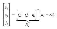
(a.8)

where 1 i and 2 i are orthonormal vectors that span Txi M and i is the unit normal to Matxi. Tosimplify the notation that follows, we let xj = (xj yj) and Xi = xj j i denote the projection of the stencil Xi to Txi M. Note that for convenience in what comes later we have shifted the coordinates so that the center of the projected stencil is xi = (00).

In the second step, the approximate Monge patch at xi is constructed from a MLS
approximant of the data (xj fj), j , which can be written as

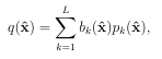
(a.9)

where {p1,….., pL is a basis for P2 (the space of bivariate polynomials of degree ) and L = dim(P2) = ( +1)( +2) 2 is the dimension of this space. The coe cients bk(x) of the approximant are determined from the data according to the weighted least squares problem

b(x) = argmin b RL sum ofj i w(xj x)(q(xj) fj)2 = argmin b RL W(x)1 2(Pb f) 2 2 (A.10)

where w : R2 R2 R 0 is a weight kernel that depends on a support parameter , W(x) is the ni ni diagonal matrix W(x) = (w(xj x)), and P is the ni L Vandermonde-type matrix

P = [p1(xj) p2(xj)], pL(xj) j i
(A.11)

Here we use underlines to denote vectors (i.e., b and f denote vectors containing coefficients and data from (B.12), respectively). Note that the coefficients bk depend on x because the kernel w depends on x (this gives origin to the term moving in MLS). We discuss the selection of the stencils and weighting kernel below, but for now it is assumed that ni > L and Xi is unisolvent on the space P2 (i.e., P is full rank), so that (B.12) has a unique solution. The MLS approximant q is used in place of f in the Monge patch (A.2) and it is used to approximate the metric terms in (A.5) (A.7). To compute these terms, various derivatives need to be approximated at the projected stencil center xi. Considering, for example, xq, the approximation is computed as follows:

(a.12)

where bk(xi) come from (B.12) with x = xi. Other derivatives of metric terms in (A.5) (A.7) are approximated in a similar way to (A.12). We note if the standard monomial basis is used for p1 pL , then by centering the projected stencil in (A.8) about the origin, only one of the derivatives of pk in (A.12) is non-zero when evaluated at xi.
Note that (A.12) is only an approximation of xq because it does not include the contribution of x(bk(x)) xi
. This approximation is referred to as a di use derivative in the literature and is equivalent to the GMLS formulation of approximating derivatives [27]. The term GMLS derivatives is preferred over diffuse derivatives to describe (A.12), since the approximation is not di use or uncertain and has the same order of accuracy as the approximations that include the derivatives of the weight kernels [26].

A.4.2 Approximating SDOs

The procedure for approximating any of the SDOs in (A.5) (A.7) is similar to the one for approximating the metric terms, but for this task we are interested in computing stencil weights as in (A.1) instead of the value of a derivative at a point. Since these SDOs involve computing various partial derivatives with respect to x and y, we can use (A.12) as a starting point for generating these stencil weights. If uj j i are samples of a function u over the projected stencil Xi, then we can again approximate xux=xi using (A.12), with bk(xi) de ned in terms of the samples of u. To write this in stencil form we note that (A.12) can be written using vector inner products as

(a.13)

where we have substituted the solution of b(xi) in (B.12) to obtain the term in the last equality. This gives the stencil weights ci x as the (weighted) least squares solution of the over determined system

W(xi)1 2Pci x = W(xi)1 2( xp(xi))
(A.14)

which is typically solved using a QR factorization of W(xi)1 2P to promote numerical
stability. Stencil weights ci y, ci xx, ci xy, and ci yy for the other derivative operators appearing in
(A.5) (A.7) can be computed in a similar manner for each stencil Xi, i = 1 N.

These can then be combined together with the approximate metric terms to define the weights cij in (A.1) for any of the SDOs in (A.5) (A.7).

A.4.3 Choosing the stencils and weight kernel

As discussed in Section A.3.1, we use Algorithm 1 to choose the stencil weights. For the initial stencil size, we use L = dim(P2). The radius factor controls the size of the stencil, with larger resulting in larger stencils, and we experiment with this parameter in the numerical results section. There are many choices for the weight kernel w in (B.12). Typically, a single radial kernel is used to de ne w as w(xy) = w( x y ), where xy Rd and is the standard Euclidean norm for Rd. In this work, we use the same family of compactly supported radial kernels as [36, 18] and implemented in [20]:

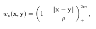(a.15)

where m is a positive integer and ()+ is the positive oor function. These C0 kernels have support over the ball of radius centered at y. While smoother kernels can be used such as Gaussians, splines, or Wendland kernels [13], we have not observed any signi cant improvement in the accuracy of GMLS derivative approximations with
smoother kernels. In general, proofs on how the choice of kernels e ects the accuracy of GMLS approximations have yet to be found. Finally, we note that the support parameter is chosen on a per stencil basis and is set equal to hmax from Algorithm 1.

A.4.4 Approximating the tangent space

When the tangent space Txi M is unknown, a coarse approximation to it can be computed for each stencil Xi using principal component analysis [22]. In this method, one computes the eigenvectors of the covariance matrix XiXT i , where Xi is the 3 by-ni matrix formed from the stencil points Xi centered about their mean. The two dominant eigenvectors of this matrix are taken as a coarse approximation to Txi M and the third is taken as a coarse approximation to the normal to M at xi; we denote these by 1 i, 2 i, and i, respectively. Next, an approximate Monge patch parameterization is formed with respect to this approximate tangent space using MLS following the same procedure outlined at the beginning of Section A.4.1. This procedure is illustrated in Figure A.3 (a), where the coarse approximate tangent plane is given in yellow. A re fined approximation to the true tangent plane and normal at the stencil center xc can be obtained by computing the tangent plane and normal to the MLS approximant of the Monge patch at xc; this plane is given in cyan in Figure A.3 (a). Once this plane is computed, a new Monge patch parameterization with respect to this re ned tangent plane approximation is formed, as illustrated in Figure A.3 (b). This procedure is repeated for each stencil Xi and the re ned tangent space computed for each stencil is used in the procedure described in Section A.4.1 for approximating the metric terms.

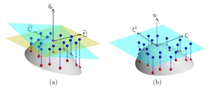
Figure A.3: Illustration of the tangent plane correction method. (a) Monge patch parameterization for a local neighborhood of a regular surface M (in gray) in 3D using a coarse approximation to the tangent plane (in yellow) at the center of the stencil xc and the re ned approximation to the tangent plane (in cyan). (b) Same as (a), but for the Monge patch with respect to the re ned tangent plane. The red spheres denote the points from the stencil and the blue spheres mark the projection of the stencil to the (a) coarse and (b) re ned tangent planes. The coarse and refined approximations to the tangent and normal vectors are given as 1 c, 2 c , and c, respectively, with tildes on these variables denoting the coarse approximation.

A.5 RBF-FD using the tangent plane

As discussed in the introduction, there are several RBF-FD methods that have been developed over the past ten years for approximating SDOs. We use the one based on the tangent plane method for formulating SDOs and PHS interpolants augmented with polynomials for approximating the derivatives that appear in this formulation. The subsections below provide a detailed overview of these respective techniques.

A.5.1 Tangent plane method

The tangent plane method similarly uses local coordinates for the surface in the tangent plane formed at each xi X, but unlike the method from Section A.4.1, it does not use approximations to the metric terms. It instead approximates the SDOs at each xi using the standard de nitions for the derivatives in the tangent plane. So, using local coordinates (A.2) about xi, the the surface gradient for the tangent plane method is taken as

(a.16)

and the surface divergence of a smooth vector u Txi M is taken as

M u= [x y 0] RT iu

(A.17)

where Ri is the rotation matrix given in (A.8). Similarly, the surface Laplacian in the tangent plane method is

M= xx+ yy
(A.18)

We next show that if Txi M is known exactly for each xi X and the point at which the SDOs are evaluated is xi, then the SDOs (A.16) (A.18) are equivalent to the corresponding ones involving metric terms (A.5) (A.7). This was shown indirectly in [11] for the surface Laplacian using the distributional deffinition of the surface Laplacian. Here we show the result follows explicitly for each surface differential operator (A.5) (A.7) from the local coordinate formulation in Section A.3.2. The rst step is to note that the vectors xf xi and yf xi from the Monge pa rameterization (A.2) are tangential to the xy-plane and must therefore be orthogonal to the vector 0 0 1 . This implies xf = yf = 0 at xi, which means the metric tensor (A.3) reduces to the identity matrix when evaluated at xi. Using this result in (A.5) for M means that the surface gradient formula (A.5) is exactly (A.16) when evaluated at xi. The equivalence of the surface divergence formulas (A.6) and (A.17) also follow immediately from this result.

The steps for showing the equivalence of the surface Laplacian operator are more involved. To simplify the notation in showing this result, we denote partial derivatives of f with subscripts. For the rst step of this process, we substitute the explicit metric terms, g= (1+f2 x)(1+f2 y) (fxfy)2, g11 = (1+fy) g, g12 = g21 = (fx)(fy) g, and g22 = (1 +fx) g, into (A.7) and expand the derivatives. Next, we simplify to obtain the following formula:

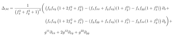
Using fx = fy = g12 = 0 and g11 = g22 = 1 at xi, this formula reduces to (A.18).

A.5.2 Approximating the SDOs

Since the tangent plane method does not require computing approximations to any metric terms, we only need to describe the RBF-FD method for approximating the derivatives that appear in (A.16) (A.18). We derive this method from derivatives of interpolants over the projected stencils for each point xi X using the same notation as Section A.4 and we assume that the tangent space is known. A method for approximating the tangent space also using RBF-FD is discussed in Section A.5.4. Let uj j i be samples of some function u over the projected stencil Xi = xj j i. The PHS interpolant to this data can be written

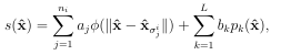
(a.19)

where (r) = r2+1 is the PHS kernel of order 2 + 1, index in i, denotes the Euclidean norm, and p1
Z 0, i j is the jth pL are a basis for P2.

The expansion coe cients are determined by the ni interpolation conditions and L additional moment conditions:

s(xj) = uj j i ni and j=1 ajpk(x i j ) = 0 k = 1 L
(A.20)

These conditions can be written as the following (ni + L) (ni + L) linear system

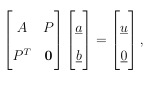(a.21)

where Ajk = x i j x i k 2+1 (jk =1 ni) and P is the same Vandermonde-type matrix given in (A.11). The PHS parameter controls the smoothness of the kernel and should be chosen such that 0 . With this restriction on , it can be shown that A is positive de nite on the subspace of vectors in Rn satisfying the L moment conditions in (B.8) [40]. Hence, if the stencil points Xi are such that rank(P) = L (i.e., they are unisolvent on the space P2), then the system (B.9) is non-singular and the PHS interpolant is well-posed. Note that this is the same restriction on Xi for the MLS problem (B.12) to have a unique solution.

The stencil weights for approximating any of the derivatives appearing in the SDOs (A.16)-(A.18) can be obtained from di erentiating the PHS interpolant (B.7). Without loss of generality, consider approximating the operator x over the stencil Xi. Using vector inner products as in (A.13), the stencil weights for this operator are determined from the approximation

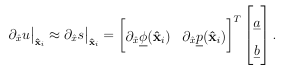
where x (xi) and xp(xi) are vectors containing the entries x x x i
j 2+1 xi , j = 1 ni, and xpk(x) xi , k = 1 L, respectively. Using (B.9) in the preceding expression gives the stencil weights as the solution to the following linear system

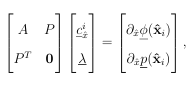
(a.22)

where the entries in are not used as part of the weights. Stencil weights ci y, ci xx, ci xy, and ci yy for the other partial derivatives can be com puted in an analogous way for each stencil Xi, i = 1,…, N. These can then be combined together to de ne the weights cij in (A.1) for any of the SDOs in (A.16) (A.18).

A.5.3 Choosing the stencils and PHS order

Similar to GMLS, we use Algorithm 1 to choose the stencils and also use the same initial stencil size of n = L for this algorithm. The parameter used to determine the PHS order should be chosen with an upper bound of (so that (B.10) is well posed) and a lower bound such that the derivatives of the PHS kernels make sense for whatever operator the RBF-FD stencils are being used to approximate. In this work we use = aswe have found that this choice works well for approximating various SDOs across a wide range of surfaces. Choosing < can be useful for improving the conditioning of the system (B.10) and for reducing Runge Phenomenon-type edge effects in RBF-FD approximations near boundaries [6].

A.5.4 Approximating the tangent space

If Txi M is unknown for any xi X, then we use a similar procedure to the one discussed for GMLS in Section A.4.4 (and illustrated in Figure A.3) to approximate it. The di erence for RBF-FD is that instead of using an MLS reconstruction of the Monge patch parameterization formed from the coarse tangent plane approximation at each xi, we use the PHS interpolant (B.7) for the reconstruction. The refined approximation to the tangent plane at each xi is then obtained from derivatives of the PHS interpolant of the Monge patch for stencil Xi. We note that this approach is new amoungst the di erent tangent plane methods, as previous approaches assumed the tangent space was computed by some other, possibly unrelated techniques, and not directly from the stencils [35, 33, 43].

A.6 Theoretical comparison of GMLS and

RBF-FD

In this section, we make comparisons of the GMLS and RBF-FD methods in terms of some of their theoretical properties, including the di erent approaches in formulating SDOs, the parameters of the approximations, and the computational cost. One of the main di erences between the GMLS and RBF-FD approaches is that the former uses the local coordinate method to formulate SDOs, while the latter uses the tangent plane method. As shown in Section B.3.1 these methods are equivalent if the tangent space for M is known for each xi X and the SDOs are evaluated at the stencil center xi. However, the GMLS method does not take advantage of this and instead includes metric terms in the formulation. These metric terms are approximated with the same order of accuracy as the GMLS approximation of the derivatives (see below), so that these errors are asymptotically equivalent as the spacing of the points in the stencil goes to zero. When the tangent space is unknown, both methods again approximate it to the same order of accuracy as their respective approximations of the derivatives.

The GMLS and RBF-FD methods each feature the parameter , which controls the degree of the polynomials used in the approximation. For a given , the formulas for either method are exact for all bivariate polynomials of degree in the tangent plane formed by the stencil center xi. Unsurprisingly, also e ects the local accuracy of the formulas in the tangent plane with increasing giving higher orders of accuracy for smooth problems; see [26, 22] for a study of the accuracy of GMLS and [10, 4] for RBF-FD. The order of accuracy of both methods depends on the highest order

derivative appearing in the SDOs, and is generally if the derivative order is 1 and 1 if the derivative order is two. However, for certain quasi-uniform point clouds with symmetries, the order has been shown to be for GMLS applied to second order operators like the surface Laplacian [22].

The computational cost of the methods can be split between the setup cost and the evaluation cost. The setup cost depends on and ni (which depends on ). For each stencil Xi, the dominant setup cost of GMLS comes from solving the ni L system (B.13), while the dominant cost for RBF-FD comes from solving the (ni + L) (ni+L) system (B.10). We use QR factorization to solve the GMLS system and LU factorization to solve the RBF-FD system, which gives the following (to leading order):

Setup cost GMLS 2sum of N i=1 n i L2 and Setup cost RBF-FD 2by3 sum of N i=1 (ni +L)3
(A.23)

The stencil sizes depend on and , and for quasi-uniform point clouds X, ni is typically some multiple of L. In this case, the setup cost of RBF-FD is higher by approximately 1 3 (1 + )3. We note that the setup procedure for both methods is an embarrassingly parallel process, as each set of stencil weights can be computed independently of every other set. The evaluation costs of both methods are the same and can be reduced to doing sparse matrix-vector products. So, for a scalar SDO like the surface Laplacian

evaluation cost GMLS & RBF-FD: 2sum of ni i=1
(A.24)

If the and parameters remain xed so that size of the stencils remain xed as N increases, then both the setup and evaluation cost are linear in N.

A.7 Numerical comparison of GMLS and
RBF-FD

We perform a number of numerical experiments comparing GMLS and RBF-FD for approximating the gradient, divergence, and Laplacian on two topologically distinct surfaces: the unit two sphere S2 and the torus de ned implicitly as

(a.25)

For the experiments with the sphere, we consider three di erent point sets X: icosa hedral, cubed-sphere and Poisson disk points. The rst two are commonly used in numerical weather prediction [8, 42] and have been used in other studies on GMLS [36] and RBF-FD [14] methods on the sphere. Unlike these rst two point sets, Poisson disk points can be generalized to other surfaces than the sphere and have also previously been used in studies on GMLS and RBF-FD methods [43]. Hence, we use Poisson disk points also for the torus and use the weighted sample elimination (WSE) algorithm [44] to generate them.

All of point sets we consider are quasi-uniform in the sense that the average spacing between the points h (or more generally the mesh-norm [13]) decreases like h N 1 2. Therefore, thesepoints sets are well-suited for testing convergence rates of GMLSandRBF-FDmethods with N (i.e., convergence as the density of the sampling of the surfaces increases). Table A.1 lists the di erent values of N used for each point set. We experimentally examine the algebraic convergence rates versus the N, assuming the error behaves like O(N 2). We include convergence rates results for polynomial degrees = 2, 4, and 6.

Node set Values of N
Icosahedral 10242, 40962, 163842, 655362
Cubed sphere 6146, 24578, 98306, 393218
Poisson disk, sphere 8192, 32768, 131072, 524288
Poisson disk, torus 8153, 32615, 130463, 521855

Table A.1: Sizes of the node sets used in the numerical experiments.

All RBF-FD results that follow were obtained from a Python implementation of the method that only utilizes the scienti c computing libraries SciPy and NumPy. For the GMLS results, we use the software package Compadre [20], which is implemented in C++ and uses the portable performance library Kokkos.

A.7.1 Convergence comparison: Sphere

We base all the convergence comparisons for the sphere on the following function consisting of a random linear combination of translates of 50 Gaussians of different widths on the sphere:

(a.26)

where yj are the centers and are selected as low discrepancy points on the sphere [9], and dj & j are sampled from the normal distributions N(01) & N(154), respectively. This function has also been used in other studies on RBF-FD methods [21]. We use samples of u in the surface gradient tests and measure the error against the exact surface gradient, which can be computed using the Cartesian gradient in R3 as Mu= u ( u),where istheunitoutward normal to S2 [16] (which is just x). Applying this to (A.26) gives

Mu=2sum of 50 j=1 dj j(yj x(x yj))exp( j x yj 2) (a.27)

We use samples of this eld in the surface divergence tests. Since M Mu = Mu, we compare the errors in this test against the exact surface Laplacian of u, which can be computed using the results of [15] as

Mu= -sum of 50 j=1 dj j(4 x yj 2(2+ j(4 x yj 2)))exp( j x yj 2)

We also use this in the tests of the surface Laplacian using samples of u. For all these tests, we set radius factor in the stencil selection Algorithm 1 to 1.5. This gave the best results for GMLS (see the next section for some results on the e ects of increasing ). While the exact tangent space for the sphere is trivially determined, we approximate it in all the results using the methods discussed in the Section A.4.4 for GMLS and Section A.5.4 for RBF-FD. These approximations are done with the same parameters for approximating the di erent SDOs to keep the asymptotic orders of accuracy comparable. Although not included here, we did experiments with the exact tangent space and obtained similar results to those presented here.

Figures A.4 A.6 display the convergence results for GMLS and RBF-FD as a function of N. Each gure is for a di erent point set type and contains the results for approximating the surface gradient, divergence, and Laplacian in both the relative two- and max-norms and for di erent polynomial degrees . We see from all the gures that the measured convergence rates for GMLS and RBF-FD are similar, but that RBF-FD gives lower errors for the same N and in almost all cases. One

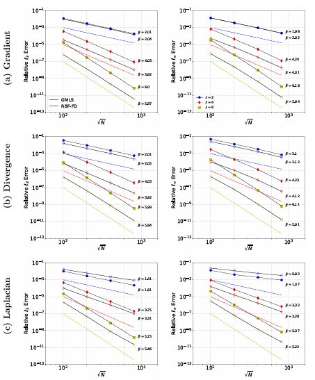
FigureA.4: Convergence results for(a)surface gradient, (b)divergence, and(b)Laplacian on the sphere using icosa hedral point sets. Errorsare given inrelative two-norms ( rst column) andmax-norms (secondcol umn). Markerscorrespondtodi erent : lledmarkersareGMLSand openmarkersareRBF-FD.Dash-dottedlineswithoutmarkerscorrespond to2nd, 4th, and6thorderconvergencewith1 N. arethemeasured orderof accuracycomputedusingthe linesofbest t tothe last three reportederrors.

notable exception is on the cubed sphere points, where the convergence rates of the max-norm errors for the GMLS approximations of the Laplacian are noticeably larger. The results in the gure also show that the measured convergence rates in the two norm for the surface gradient and divergence approximations are close to the expected rates of for all the point sets. However, when looking at the convergence rates of the surface Laplacian, we see from Figures A.4 & A.5 that the icosahedral and cubed sphere points have higher rates than for the Poisson disk points in Figure A.6. These improved convergence rates have been referred to as superconvergence in the GMLS literature and rely on the point set being structured so that the stencils have certain symmetries [22]. When these symmetries do not exist, as is the case for the Poisson disk points, then the convergence rates for the surface Laplacian follow more closely the expected rates of 1

A.7.2 Convergence comparison: Torus

The convergence comparisons on the torus are based on the target function

u(x) = x 8 (x4 10x2y2 +5y4)(r2 60z2) x T2
(A.28)

where r = x2+y2. This function has also been used in other studies of RBF methods for surfaces [16]. As with the sphere example, the surface gradient of u can be computed as Mu = u ( u),where isthe unit outward normal to T2, which can be computed from the implicit equation (A.25). The surface Laplacian of (A.28) is given in [16] as

Mu(x) = 3x 8r2 (x4 10x2y2 +5y4)(10248r4 34335r3 +41359r2 21320r +4000) x T2.

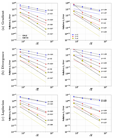
Figure A.5: Same as Figure A.4,but for the cubed sphere points.

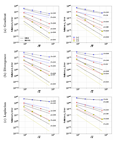
FigureA.6: Same as FigureA.4,but for the Poisson disk point son the sphere.

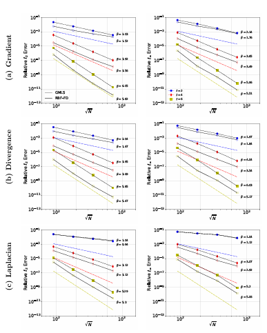
FigureA.7: Same as FigureA.4, but for to rus using Poisson disk points.

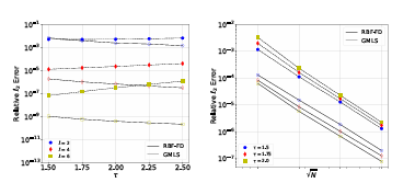
Figure A.8: Relative two-norm errors of the surface Laplacian approximations as the stencil radius parameter varies. Left gure shows errors for several di erent values of and a xed N = 130463. Right gure shows the convergence rates of the methods for di erent and a xed = 4.

Similar to the sphere, we use samples of Mu in the tests of the divergence and
compare the results with Mu above. We rst study the convergence rates with the stencil radius scaling = 15 and approximate the tangent space, as we did with the sphere tests. Figure A.7 displays the results for the surface gradient, divergence, and Laplacian. We see that errors for RBF-FD are again smaller than the errors for GMLS in almost all cases over the range of N tested. However, GMLS has a slightly higher convergence rates in the case of the surface gradient and divergence, but not for the Laplacian. Both methods have convergence rates that are close to the expected rates of for these surface gradient and divergence and 1 for the Laplacian.

Next we investigate how the approximation properties of the two methods change when is increased, which results in larger stencil sizes. We focus on approximating the surface Laplacian as similar results were found for the other SDOs. In the left plot of Figure A.8, we show the relative two-norm errors of the approximations for a

fixed N as varies from 1.5 to 2.5. We see that increasing has opposite e ects on the two methods: the errors decrease for RBF-FD and increase with GMLS. We see similar results in the right plot of Figure A.8, where we show the convergence of the methods with increasing N for di erent xed values of (and xed at 4). While the convergence rates do not appear to change with , the overall errors decrease for RBF-FD and increase for GMLS. These results make sense when one considers the di erent types of approximations the methods are based on: RBF-FD is based on interpolation, while GMLS is based on least squares approximation. As the stencil sizes increase, RBF-FD has a larger approximation space consisting of more shifts of PHS kernels, which can reduce the errors [10]. However, GMLS has the same xed approximation space of polynomials of degree regardless of the stencil size. This gives another parameter that can be tuned for RBF-FD to give better results for the same xed polynomial degree.

Finally, we compare the errors when the exact and approximate tangent spaces are used in the two methods. We focus only on the surface Laplacian and for = 4 since similar results were obtained for the other operators and other . Table A.2 shows the results for both methods. The approximate tangent spaces were computed using the methods from Sections A.4.4 (GMLS) and A.5.4 (RBF-FD) also using the polynomial degree = 4. We see from the table that the differences between using the exact or the approximate tangent spaces is minor.

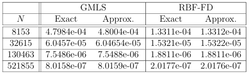
Table A.2: Comparison of the relative 2 errors for the surface Laplacian on the torus using the exact tangent space for the torus and approximations to it based on the methods from Sections A.4.4 (GMLS) and A.5.4 (RBF FD). In all cases, = 4 and the points are based on Poisson disk sampling.

A.7.3 E ciency comparison

The results in Section B.6 demonstrate that RBF-FD and GMLS have similar asymptotic convergence rates for the same , but that RBF-FD can achieve lower errors for the same N and stencil sizes. In this section, we consider which of the methods is more computationally e cient in terms of error per computational cost. We examine both the effciency when the setup costs are included and when just the evaluation costs are included, as measured by (A.23) and (A.24), respectively. We limit this comparison to = 15 since this gave the best results for GMLS. Figure ?? displays the results of this examination for the case of computing the surface Laplacian on the tours discretized with Poisson disk sampling. Similar results were obtained for other SDOs and for the sphere, so we omit them. We see from the gure that GMLS is more e cient when the setup costs are included, but that RBF-FD is more e cient when only evaluation costs are included. For problems where the point sets are xed and approximations to a SDO are required to be performed multiple times as occurs when solving a time-dependent surface PDEs the setup costs are not as important as the evaluation costs since they are amortized across all time-steps. In this scenario RBF-FD is the more efficient method.

A.8 Concluding remarks

We presented a thorough comparison of the GMLS and RBF-FD methods for ap proximating the three most common SDOs: the gradient, divergence, and Laplacian (Laplace-Beltrami). Our analysis of the two di erent formulations of SDOs used in the methods revealed that if the exact tangent space for the surface is used, these for
mulations are identical. Our numerical investigation of the methods showed that they appear to converge at similar rates when the same polynomial degree is used, but that RBF-FD generally gives lower errors for the same N and . We further examined the dependency of the stencil size on the methods (as measured by the parameter) and found that the errors produced by GMLS deteriorate as the stencil size increases.

The errors for RBF-FD, contrastingly, appear to keep improving as the stencil size increases. However, we dont expect this trend to continue inde nitely, as eventually the tangent plane formulation breaks down when the stencil size becomes too large.

Finally, we investigated the computational e ciency of the methods in terms of error versus computational cost and found GMLS to be more e cient when setup costs are included and RBF-FD to be more e cient when only considering evaluation costs.

Acknowledgements

AMJ was partially supported by US NSF grant CCF-1717556. PAB & PAK were supported by the U.S. Department of Energy, O ce of Science, Advanced Scienti c Computing Research (ASCR) Program and Biological and Environmental Research (BER) Program under a Scienti c Discovery through Advanced Computing (SciDAC 4) BERpartnership pilot project. PAK was additionally supported by the Laboratory Directed Research & Development (LDRD) program at Sandia National Laboratories and ASCR under Award Number DE-SC-0000230927. AMJ was also partially supported by the Climate Model Development and Validation (CMDV) program, funded by BER. Part of this work was conducted while AMJ was employed at the Computer Science Research Institute at Sandia National Laboratories. GBW was partially supported by U.S. NSF grants CCF-1717556 and DMS-1952674.

This paper describes objective technical results and analysis. Any subjective views or opinions that might be expressed in the paper do not necessarily represent the views of the U.S. Department of Energy or the United States Government. Sandia National Laboratories is a multimission laboratory managed and operated by National Technology & Engineering Solutions of Sandia, LLC, a wholly owned subsidiary of Honeywell International Inc., for the U.S. Department of Energys National Nuclear Security Administration under contract DE-NA0003525. SAND2022-XXXXJ.

REFERENCES

[1] Alvarez, Diego, Gonzalez-Rodrguez, Pedro, and Kindelan, Manuel. 2021. A Local Radial Basis Function Method for the LaplaceBeltrami Operator. J. Sci. Comput., 86(3), 28.

[2] Banerjee, Sanjoy, Lakehal, Djamel, and Fulgosi, Marco. 2004. Surface divergence models for scalar exchange between turbulent streams. International Journal of Multiphase Flow, 30(7), 963977. A Collection of Papers in Honor of Professor G. Yadigaroglu on the Occasion of his 65th Birthday.

[3] Bayona, Victor. 2019a. Comparison of Moving Least Squares and RBF+Poly for Interpolation and Derivative Approximation. J. Sci. Comput., 81(1), 486512.

[4] Bayona, Vctor. 2019b. An insight into RBF-FD approximations augmented with polynomials. Comput. Math. Appl., 77(9), 23372353.

[5] Bayona, Victor, Flyer, Natasha, Fornberg, Bengt, and Barnett, Gregory A. 2017. On the role of polynomials in RBF-FD approximations: II. Numerical solution of elliptic PDEs. J. Comput. Phys., 332, 257273.

[6] Bayona, Vctor, Flyer, Natasha, and Fornberg, Bengt. 2019. On the role of poly nomials in RBF-FD approximations: III. Behavior near domain boundaries. J. Comput. Phys., 380, 378 399.

[7] Bertalmo, M., Cheng, L., Osher, S., and Sapiro, G. 2001. Variational problems and partial di erential equations on implicit surfaces. J. Comput. Phys., 174, 759780.

[8] Bosler, P.A., Wang, L., Jablonowski, C., and Krasny, R. 2014. A Lagrangian particle/panel method for the barotropic vorticity equations on a rotating sphere. Fluid Dyn. Res., 46.

[9] Cui, Jianjun, and Freeden, Willi. 1997. Equidistribution on the Sphere. SIAM J. Sci. Stat. Comput, 18, 595 609.

[10] Davydov, Oleg, and Schaback, Robert. 2019. Optimal stencils in Sobolev spaces. IMA J. Num. Analy., 39(1), 398422.

[11] Demanet, Laurent. 2006. Painless, highly accurate discretizations of the Lapla cian on a smooth manifold. Technical report, Stanford University.

[12] Dziuk, Gerhard, and Elliott, Charles M. 2013. Finite element methods for surface PDEs. Acta Numerica, 22, 289396.

[13] Fasshauer, G. E. 2007. Meshfree Approximation Methods with MATLAB, Inter disciplinary Mathematical Sciences. Singapore: World Scienti c Publishers.

[14] Flyer, N., Lehto, E., Blaise, S., Wright, G. B., and St-Cyr, A. 2012. A guide to RBF-generated nite di erences for nonlinear transport: shallow water simulations on a sphere. J. Comput. Phys., 231, 40784095.

[15] Fornberg, Bengt, and Flyer, Natasha. 2015. A Primer on Radial Basis Functions with Applications to the Geosciences. Philadelphia, PA, USA: Society for Industrial and Applied Mathematics.

[16] Fuselier, Edward J, and Wright, Grady B. 2013. A high-order kernel method for diffusion and reaction-di usion equations on surfaces. J. Sci. Comput., 56(3), 535565.

[17] Gowan, Evan J., Zhang, Xu, Khosravi, Sara, Rovere, Alessio, Stocchi, Paolo, Hughes, Anna L. C., Gyllencreutz, Richard, Mangerud, Jan, Svendsen, John-Inge, and Lohmann, Gerrit. 2021. A new global ice sheet reconstruction for the past 80000 years. Nature Communications, 12(1), 1199.

[18] Gross, B. J., Trask, N., Kuberry, P., and Atzberger, P. J. 2020. Meshfree methods on manifolds for hydrodynamic ows on curved surfaces: A Generalized Moving Least-Squares (GMLS) approach. J. Comput. Phys., 409, 109340.

[19] Gunderman, David, Flyer, Natasha, and Fornberg, Bengt. 2020. Transport schemes in spherical geometries using spline-based RBF-FD with polynomials. J. Comput. Phys., 408, 109256.

[20] Kuberry, Paul, Bosler, Peter, and Trask, Nathaniel. 2019 (Jan.). Compadre Toolkit.

[21] Lehto, E, Shankar, V, and Wright, G. B. 2017. A radial basis function (RBF) compact nite di erence (FD) scheme for reaction-di usion equations on surfaces. SIAM J. Sci. Comput., 39, A219A2151.

[22] Liang, Jian, and Zhao, Hongkai. 2013. Solving Partial Di erential Equations on Point Clouds. SIAM J. Sci. Comput., 35(3), A1461A1486.

[23] Liu, Jinghui, Totz, Jan F., Miller, Pearson W., Hastewell, Alasdair D., Chao, Yu-Chen, Dunkel, Jorn, and Fakhri, Nikta. 2021. Topological braiding and virtual particles on the cell membrane. Proc. Natl. Acad. Sci. U.S.A., 118(34).

[24] Mahadevan, Vijay S, Guerra, Jorge E, Jiao, Xiangmin, Kuberry, Paul, Li, Yipeng, Ullrich, Paul, Marsico, David, Jacob, Robert, Bochev, Pavel, and Jones, Philip. 2022. Metrics for Intercomparison of Remapping Algorithms (MIRA) pro tocol applied to Earth system models. Geosci. Model Dev., 15(17), 66016635.

[25] Mikkelsen, Morten S. 2020. Surface GradientBased Bump Mapping Framework. Journal of Computer Graphics Techniques (JCGT), 9(4), 6091.

[26] Mirzaei, Davoud. 2016. Error bounds for GMLS derivatives approximations of Sobolev functions. J. Comput. Appl. Math, 294, 93101.

[27] Mirzaei, Davoud, Schaback, Robert, and Dehghan, Mehdi. 2011. On generalized moving least squares and di use derivatives. IMA J. Numer. Anal., 32, 9831000.

[28] O neill, Barrett. 2006. Elementary Di erential Geometry. Second edn. Elsevier.

[29] Petras, Argyrios, Ling, Leevan, and Ruuth, Steven J. 2018. An RBF-FD closest point method for solving PDEs on surfaces. J. Comput. Phys., 370, 4357.

[30] Piret, Cecile, and Dunn, Jarrett. 2016. Fast RBF OGr for solving PDEs on arbitrary surfaces. AIP Conference Proceedings, 1776(1), 070005.

[31] Shankar, Varun, Wright, Grady B., Kirby, Robert M., and Fogelson, Aaron L. 2014. A Radial Basis Function (RBF)-Finite Di erence (FD) Method for Di usion and Reaction-Di usion Equations on Surfaces. J. Sci. Comput., 63(3), 745 768.

[32] Shankar, Varun, Narayan, Akil, and Kirby, Robert M. 2018. RBF-LOI: Augment ing Radial Basis Functions (RBFs) with Least Orthogonal Interpolation (LOI) for solving PDEs on surfaces. J. Comput. Phys., 373, 722735.

[33] Shaw, Sage. 2019. Radial Basis Function Finite Di erence Approximations of the Laplace-Beltrami Operator. M.Phil. thesis, Boise State University, USA. 1587.

[34] Stoop, Norbert, Lagrange, Romain, Terwagne, Denis, Reis, Pedro M, and Dunkel, Jorn. 2015. Curvature-induced symmetry breaking determines elastic surface patterns. Nature Materials, 14(3), 337342.

[35] Suchde, Pratik, and Kuhnert, Jorg. 2019. A meshfree generalized nite di erence method for surface PDEs. Comp. Math. Appl., 78(8), 27892805.

[36] Trask, Nathaniel, and Kuberry, Paul. 2020. Compatible meshfree discretization of surface PDEs. Computational Particle Mechanics, 7, 271277.

[37] Trask, Nathaniel, Perego, Mauro, and Bochev, Pavel. 2017. A high-order stag gered meshless method for elliptic problems. SIAM J. Sci. Comput., 39(2), A479 A502.

[38] Vallis, Geo rey K. 2006. Atmospheric and Oceanic Fluid Dynamics: Fundamentals and Large-scale Circulation. Cambridge University Press.

[39] Walker, Shawn W. 2015. The Shapes of Things. Philadelphia: Society for Industrial and Applied Mathematics.

[40] Wendland, Holger. 2005. Scattered Data Approximation. Vol. 17. Cambridge: Cambridge University Press.

[41] Wendland, Holger, and Kunemund, Jens. 2020. Solving partial di erential equations on (evolving) surfaces with radial basis functions. Advances in Computational Mathematics, 46, 64.

[42] Williamson, David L. 2007. The Evolution of Dynamical Cores for Global At mospheric Models. J. Meteorol. Soc. Jpn., 85B, 241269.

[43] Wright, G. B., Jones, A. M., and Shankar, V. 2022. MGM: A meshfree geometric multilevel method for systems arising from elliptic equations on point cloud surfaces. SIAM J. Sci. Comput., Accepted.

[44] Yuksel, Cem. 2015. Sample Elimination for Generating Poisson Disk Sample Sets. Computer Graphics Forum (Proceedings of EUROGRAPHICS 2015), 34(2), 25 32.

APPENDIX B:
PAPER 2: MGM: A MESHFREE GEOMETRIC
MULTILEVEL METHOD FOR LINEAR
SYSTEMS ARISING FROM ELLIPTIC
EQUATIONS ON POINT CLOUD SURFACES

Authors: Grady B. Wright, Andrew M. Jones, Varun Shankar

B.1 Abstract

We develop a new meshfree geometric multilevel (MGM) method for solving linear systems that arise from discretizing elliptic PDEs on surfaces represented by point clouds. The method uses a Poisson disk sampling-type technique for coarsening the point clouds and new meshfree restriction/interpolation operators based on polyharmonic splines for transferring information between the coarsened point clouds. These are then combined with standard smoothing methods in a V-cycle iteration. MGM is applicable to discretizations of elliptic PDEs based on various localized meshfree methods, including RBF nite di erences (RBF-FD) and generalized nite di erences (GFD). We test MGM both as a standalone solver and preconditioner for Krylov sub space methods on several test problems using RBF-FD and GFD, and numerically analyze convergence rates, e ciency, and scaling with increasing point cloud sizes. We also perform a side-by-side comparison to algebraic multigrid (AMG) methods for solving the same systems. Finally, we further demonstrate the e ectiveness of MGM by applying it to three challenging applications on complicated surfaces: pattern formation, surface harmonics, and geodesic distance.

B.2 Introduction

Partial di erential equations (PDEs) de ned on surfaces (or manifolds) arise in many areas of science and engineering, where they are used to model, for example, atmospheric ows [50], chemical signaling on cell membranes [28], morphogenesis [42], and textures for computer graphics [46]. Solutions of these models can rarely be achieved by analytical means and must instead be approximated using numerical techniques. While numerical methods for PDEs on the sphere have been developed since the 1960s [50], development of methods for PDEs on more general surfaces only began in the late 1980s [15], with interest growing considerably in the early 2000s [16].

These techniques include surface nite element (SFE) [16], embedded nite element (EFE) [8? ], and closest point (CP) [29] methods. More recently, various meshfree (or meshless) methods have also been developed for PDEs on general surfaces that use a local stencil approach, including radial basis function- nite di erences (RBF FD) [2, 26, 39, 35, 40, 48], generalized nite di erences (GFD) [43], and generalized moving least squares (GMLS) [27, 44, 20]. These methods can be applied for surfaces represented only by point clouds and do not require a surface triangulation like SFE methods or a level-set representation of the surface like EFE methods. Additionally, these meshfree methods approximate the solutions directly on the point cloud and do not extend the PDEs into the embedding space like the EFE and CP methods.

In this paper, we concentrate on local meshfree methods for elliptic PDEs on surfaces, which are challenging to solve with iterative methods because of the poor conditioning of the systems. We speci cally focus on the surface Poisson and shifted (or screened) surface Poisson problems, which, for example, in surface hydrodynamics [20], computer graphics [36], and time-implicit discretizations of surface reaction di usion equations [39]. We focus on two methods for these PDEs: polyharmonic spline-based RBF-FD with polynomials and GFD. These meshfree discretizations re sult in large, sparse, non-symmetric, linear systems of equations that need to be solved. Direct solvers for these systems have most commonly been used, but these do not scale well to large point clouds and high-orders of accuracy, motivating the need for efficient and robust iterative methods. Multigrid methods are known to be e ective solvers and preconditioners for linear systems that arise from discretizing elliptic PDEs (e.g., [45]). These methods can be classi ed into two types: geometric and algebraic. While algebraic multigrid (AMG) methods are general purpose solvers/preconditioners, geometric methods, when they can be developed, generally converge faster and work as better preconditioners for Krylov subspace methods. Geometric multigrid methods have been developed for SFE and CP discretizations (e.g., [24] and [10]) and it is the aim of this paper to also develop these methods for meshfree discretizations.

The basic components of geometric multigrid methods that need to be developed are (1) techniques for coarsening the grid or mesh, (2) constructing interpolation/restriction operators for transferring the information between levels, (3) discretizing the di erential operator on the coarser levels, (4) smoothing the approximate solution, and (5) solving the system of the coarsest level. The rst component presents a challenge for meshfree surface PDEs as there is only a point cloud available and no grid or mesh to create a hierarchy of coarser levels.

To overcome this challenge we use the weighted sample elimination (WSE) method from [52], which is a general purpose method for selecting quasi-uniformly spaced subsets of points from a point cloud and falls into the general category of Poisson disk sampling methods [9]. The lack of a grid or mesh also presents a challenge for component (2) as standard transfer operators cannot be used. To overcome this challenge, we use RBFs to construct the interpolation operators for transferring the defect from coarser to ner levels. For the restriction operators, we simply use the transpose of the interpolation operators, which is a standard choice [45]. With these transfer operators, we generate component (3) using a Galerkin projection, often referred to as the Galerkin coarse grid operator. Finally, for component (4) we use standard Gauss-Seidel smoothing and for (5) we use a direct solver. We combine all of these components in a V-cycle iteration and apply it both as a solver and preconditioner. The resulting method is entirely meshfree and we refer to it as the meshfree geometric multilevel1 (MGM) method.

The new MGM method has some similarities to the meshfree multicloud meth ods [22, 54], but also some key di erences. The rst major di erence is that multicloud methods have been developed for PDEs posed in planar domains, whereas MGM is for surface PDEs. Another di erence is with the choice of transfer operators. The method of [54] uses one-point, piecewise constant operators, while the method of [22] uses two-point, inverse-distance weighted interpolation and restriction operators. It is not clear how these latter transfer operators should be generalized to surfaces. MGM instead uses transfer operators based on RBFs, which are well suited for interpolation on surfaces [17]. A second di erence is the strategy for geometric coarsening of the given point cloud. Multicloud methods use a graph coloring-type scheme for nding maximally-independent subsets of vertices to determine the coarser levels.

This does not allow the size of the point clouds on the coarser levels to be controlled precisely, and it limits the coarsening factors to approximately four (for 2D problems). MGM instead uses WSE [52], which allows for arbitrary coarsening factors and for the sizes of the points in the coarser levels to be controlled exactly. A third di erence is that MGM can handle degenerate PDEs (e.g., the surface Poisson equation), while the multicloud methods have been tailored to non-degenerate PDEs (e.g. planar Poisson equation with mixed Dirichlet-Neumann boundary conditions). Finally, multicloud methods have only been tested on second order accurate discretizations of PDEs; these discretizations typically only use small stencils. We demonstrate that MGM 1We use the term multilevel rather than multigrid, since this method does not depend on a grid.

works for discretizations at least up to sixth order accurate with large stencil sizes. The remainder of the paper is organized as follows. In Section B.3, an overview is given of the two meshfree methods for surface PDEs that the MGM algorithm is used to solve. The next section presents the RBF-based transfer operators. Section B.5 describes the remaining components of the MGM algorithm, including a discussion of the changes necessary to solve the degenerate surface Poisson problem. Section B.6 presents an extensive array of numerical results for the MGM method, including a comparison with algebraic multigrid (AMG) methods. Section B.7 then uses the method in three challenging applications to further demonstrate its e ectiveness. Finally, the paper concludes with some nal remarks on the method and some future directions in Section B.8.

B.2.1 Assumptions and notation

Throughout the manuscript we let M beasmoothembeddedmanifoldofco-dimension one in 3 with no boundary and let M denote the Laplace-Beltrami operator (LBO) (or surface Laplacian) on M. When referencing points on M, we assume they are represented as coordinates in R3, e.g., for x M, and we write x = (xy z). For a point x M, we let TxM denote the tangent plane to M at x. We denote normal vectors to M as n and assume that they are available either analytically or using some approximation technique (see for example [23]). We use sub/superscripts h and H on variables to indicate whether they are associated with the ne or coarse level point clouds, respectively. For example, Xh and XH denote the set of points in the ne level and coarse level point clouds, respectively.

This is meant to mimic the notation that is used in traditional grid based geometric multigrid methods [45], but these parameters do not relate to anything speci c about the spacing of the points and do not need to be computed.
The focus of this study is on the elliptic equation

Lu =f (B.1)

where u : M R is unknown and f : M R is known. Here L = M or L =I M , where I is the identity operator and > 0, which correspond to the surface Poisson and shifted (or screened) surface Poisson equation (B.1), respectively. For the surface Poisson problem, we assume f satis es the compatibility condition M fdA=0,whichisanecessary and su cient condition for (B.1) to have a solution.

In this case, any solution is unique up to the addition of a constant since constants satisfy the homogeneous equation.

B.3 Localized meshfree discretizations

Several localized meshfree methods have been developed for approximating the solution of (B.1), e.g., [27, 44, 2, 26, 39, 35, 40]. For the sake of brevity, we limit the focus of this study to two localized meshfree methods: polyharmonic spline (PHS) based RBF-FD with polynomials and GFD. Both of these methods use the so-called tangent plane approach, but di er in the approximation spaces used. They should be sufficient to demonstrate the general applicability of the MGM method.

The RBF-FD and GFD methods are based on approximating the strong form of the equation, and amount to discretizing the LBO M over a local stencil of points on the surface. This stencil based approach can generally be described as follows. Let Xh = xi Nh i=1 denote the global point cloud (node set) discretizing M. For each xi Xh, i = 1 Nh, let h i denote the set of indices of the ni > 1 nearest neighbor nodes in Xh to xj. Here we use the Euclidean distance in 3 to de ne the nearest neighbor distances. The points Xi h = xj j h i are the stencil for xi, and xi is the stencil center. The stencil based approximation to Mu at xj then takes the form

where cij are some set of weights determined by the RBF-FD or GFD methods dis cussed below. These weights can then be assembled into a global Nh-by-Nh (sparse) differentiation matrix Dh and an approximate solution to (B.1) is given as a solution to the linear system

Lhuh = fh
(B.3)

where uh fh RNh contain the unknown solution and known right hand side of (B.1), respectively, sampled at Xh. The matrix Lh is given by Lh = Dh or Lh = Ih Dh, where Ih is the Nh-by-Nh identity matrix. Note that the latter Lh arises from time implicit discretizations of surface di usion-type problems. The MGM method will be used for solving the system (B.3). In the remainder of this section, we give speci c details on determining the stencil weights in (B.2) for the LBO using RBF-FD and GFD methods. Since both of these methods use the tangent plane technique, we review it rst.

B.3.1 Tangent plane method

The tangent plane idea was introduced by Demanet [13] and recently further re fined by Suchde & Kuhnert [43], Shaw [41], and, in the case of the unit two-sphere, by Gunderman et. al. [21]. The central idea of the method is to approximate the LBO at the center of each stencil Xi h using an approximation to the standard Laplacian on the plane tangent to the surface at the stencil center, Txi M. The approximation is constructed from a projection of the stencil points to Txi M. In this work, we use the projection advocated in [43], which is known as an orthographic projection when Mis the unit sphere.

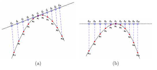
Figure B.1: Illustration of the tangent plane method for a 1D surface (curve). The solid black lines indicates the surface, the solid red circles mark the n = 11 stencil nodes, the open blue circles mark the projected nodes, and the s marks the stencil center. (a) Direct projection of the stencil points according to (B.4). (b) Rotation and projection of the stencil points according to (B.6).

With out loss of generality, we describe the method for the rst stencil X1 h with index set 1 h. To simplify notation, we assume 1 h = 1 points are simply X1 h = x1 n , so that the stencil xn . The tangent plane method from [43] projects
these points onto Tx1 M along the normal vector n1 (the normal to the surface at x1). This projection is illustrated in Figure B.1 (a) for a one dimensional surface (curve) in 2. The projected points can be computed explicitly by

j =(I n1nT 1)(xj x1) j =1,…., n (b.4)

where we have shifted the projected points so that 1 is at the origin. For a two dimensional surface, the projected points can be expressed in terms of orthonormal vectors t1 and t2 that span Tx1 M as follows

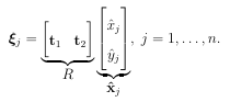
(b.5)

The 2D coordinates xj in the tangent plane for the projected points are what will be used for constructing the approximations to the Laplacian. These can be computed directly from the relationship (B.4) and (B.5) as

xj = RT(xj x1) j =1 n (b.6)

where we have used RT(I n1nT 1) = RT. We denote the the projected stencil as X1 h = x1 xn . The above procedure is repeated for every stencil Xi h, to obtain the projected stencils Xi h, i = 1 Nh.

We note that, geometrically speaking, (B.6) amounts to rst shifting the stencil points so the center is at the origin, rotating them so the normal n1 is orthogonal to the xy-plane, and then dropping the third component. This is illustrated in Figure B.1 (b) for the case of a 1D curve.

B.3.2 PHS-based RBF-FD with polynomials

The RBF-FD method for determining the weights in (B.2) can be derived by constructing an RBF interpolant over each of the projected stencil points to the tanget plane, applying the standard 2D Laplacian to the interpolants, and then evaluating them at the stencil center. In this study we focus on interpolants constructed from PHS kernels and polynomials [5, 14, 41]. Without loss of generality, we again describe the method for the rst stencil, with X1,…,
h = x1 xn , to simplify notation. For the stencil X1 h, the PHS interpolant to the projected stencil X1 h takes the form

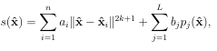
(b.7)

where x =[ x y] tx m, denotes the Euclidean norm, k is the order of the pL is a basis for bivariate polynomials in Tx1
M of degre (so that L = ( +1)( +2) 2). The order k controls the smoothness of the PHS and is chosen such that 0 k
. We note that the polynomials can be chosen to be the standard bivariate monomials in the components of x. For samples u1 un of an arbitrary function at the stencil points X1 h, the coe cients for the interpolant in the tangent plane are determined by the conditions

(b.8)

which can be written as the following linear system

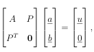
(b.9)

whereAij= xi xj 2k+1 (i j=1 n),Pij=pj(xi)(i=1 n, j=1 L), and underline dterms denote vectors containing the corres ponding termsin(B.8). If thestencilnodesX1 hareunisolventwithrespecttothespaceofbivariatepolynomials ofdegree (i.e.,rank(P)=L),then(B.9)hasauniquesolution,sothat(B.7)iswell posed[47]. This isamildconditiononthestencilnodes, especiallyfor scattered nodesonthetangentplane. The stencilweightsc1j in(B.2)are determined from the approximation

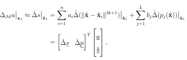
where = xx+ yy, sand pare vectors containing the entries ( x xi 2k+1) x1 , i=1 n, and (pj(x)) x1
, j=1 L, respectively. Using(B.9) in the abov expression, the stencil weight saregiven as the solution to the following linear system

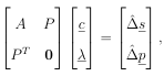
(b.10)

whereccontainsc1j and areun used.

We note that one can interpret (B.10) as the solution to an equality constrained optimization problem where the weights are determined by enforcing they are exact for ( x xi 2k+1) x1 , j = 1 for (pj(x)) x1 , j = 1 multipliers [5]. n, subject to the constraint that they are also exact L. Under this interpretation, is the vector of Lagrange In this work, we choose the order of the PHS as k = and xthestencilsize nj = n, j =1 Nasn= 2L,whichis a common choice for RBF-FD methods [5]. The degree of the appended polynomial can then be used to control the approximation order of the method, with larger leading to higher orders [12].

B.3.3 GFD

This method is similar to the RBF-FD method, but instead of using an interpolant, the method is based on a (weighted) polynomial least squares approximant. Using the same notation and assumptions as the previous section and again focusing only on the rst stencil X1 h, the approximant for the projected stencil X1 h takes the form

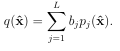
(b.11)

The coe cients of the approximant are determined from the samples u1,…., according to the the following weighted least squares problem:

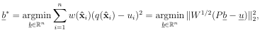
(b.12)

where W = (w(xi)). Here we again assume the stencil nodes X1 h are unisolvent with respect to bivariate polynomials of degree L so that (B.12) has a unique solution. There are many different options for selecting the weight function w in the literature. In this work, we follow [43] and use the following Gaussian function:

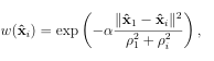
where k is the support of the kth projected stencil Xi h, i.e. the radius of the minimum ball centered at xi that encloses all the points in Xi h. The parameter > 0 is used for controlling the shape of the weight function and is typically chosen in an ad hoc manner [43].
The stencil weights in (B.2) are determined from the approximation

Using the normal equation solution of (B.12) in the above expression, the vector of stencil weights c is given as

c =WP(PTWP) 1( p) (b.13)

(b.14)

In practice, a QR factorization of WP is used instead of the normal equations to improve the numerical conditioning of (B.13). In this work, we choose the number of points in the stencils Xi h for this method in the same manner as the RBF-FDtechnique. Note that, similar to RBF-FD, increasing the polynomials degree also increases the order of accuracy of the GFD method.

B.4 Multilevel transfer operators using RBFs

Operators for transferring information between coarse and ne levels are one of the key components of multilevel methods. The interpolation transfer operators are used to transfer information from coarse level to a ner level, while the restriction operators are used for the reverse. Let Xh = xi Nh i=1 Mdenote the ne set of nodes and
XH = yj NH j=1 M the coarse set, where NH < Nh. We denote the interpolation operator by Ih
H and the restriction operator by IH h . These can be represented of as (sparse) matrices, so that for a vector uH of data on the coarse nodes XH, the vector containing the interpolation of uH to Xh is given as uh = Ih
HuH. In this section, we discuss a novel meshfree method for constructing Ih H based on RBF interpolation. For
the restriction operator, we use IH h = (Ih H)T, which is a standard choice, especially in AMG methods [45, Appendix A]. Similar to the discrete LBO, we compute the interpolation operator using a stencil based approach. Letting i H be the indicies of the mi nearest neighbors in XH to xi, the interpolation of uH j j H
i to uh i, the entry in uh corresponding to xi, is given as

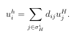
(b.14)

We again use the Euclidean distance in R3 to de ne the index set i H. The weights for each stencil can be assembled to form the (sparse) interpolation matrix Ih H. We use local RBF interpolants about each stencil Xi
H = yj j H i to determine the weights in (B.14) and form these interpolants in the embedding space R3. This is con siderably simpler than using intrinsic coordinates to M and the resulting interpolants have good approximation properties [17]. One could alternatively use interpolants in the tangent plane about each stencil center similar to Section B.3.2, but these are only accurate when the surface is well discretized by the underlying point cloud. This will not necessarily be the case for the nodes XH as we coarsen the the ner levels. We again use a PHS kernel to form the interpolants and describe the method for the rst stencil X1 H, which, to simplify the notation, we assume to consist of the nodes y1 ym . For the stencil X1 H, the PHS interpolant takes the same form as (B.7), but with x replaced by x and xi is replaced by yi . Additionally, we only consider the PHS kernel with k = 0 and a constant term appended to the interpolant (i.e. = 0). The weights d1j in (B.14) are determined by evaluating this interpolant at x1 and can be computed in a similar procedure to that used in deriving the system (B.10). The linear system for the interpolation weights takes the form

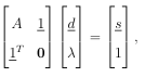
(b.15)

where Aij = yi yj (i j = 1 ,….., m), 1 is the vector of length n with all ones, and s has entries x1 yi , i = 1 m. Again, is unused. While higher order PHS kernels (k > 0) and higher degree polynomials ( > 0) could be used in constructing the interpolation weights, we found that the simple for mulation above gave good results, while also being e cient, for the range of problems we considered. This formulation also has the added bene t that the system (B.15) has a unique solution, provided the points are distinct [47]. When using larger k and this may not be the case as the points must be unisolvent with respect to the space of trivariate polynomials of degree , i.e., (P) = L. Since the interpolation is done

Algorithm 2: Two-Level Cycle

1 Pre-smooth initial guess: uh presmooth(Lh uh fh 1);
2 Compute residual: rh = fh Lhuh;
3 Restrict the residual to XH: rH = IH hrh;
4 Solve for the defect: LHeH = rH;
5 Interpolate the defect to Xh: eh = Ih HeH;
6 Correct the approximation: uh uh +eh;
7 Post-smooth the approximation: uh postsmooth(Lh uh fh 2);

in the embedding space, this can be an issue for certain algebraic surfaces (e.g., the sphere with 2).

B.5 Meshfree geometric multilevel (MGM)
method

In this section we present the MGM method for solving the discrete problem (B.3). We rst present the MGM method in terms of a two-level cycle, which is summarized in Algorithm 2, describing its primary components: coarsening the point cloud Xh XH, forming the coarse level operator LH, smoothing the approximation, and solving for the defect on the coarse level. The interpolation/restriction operators are described in the previous section. We then focus on some modi cations to the algorithm that are necessary when (B.3) corresponds to the surface Poisson problem.

This is followed by a description of the multilevel extension of the method. Finally, we comment on using the method as a preconditioner for Krylov subspace methods.

B.5.1 Node coarsening

The technique we propose for generating the coarser point clouds on general surfaces is based on (WSE) method from [52]. This algorithm falls into the category of Poisson disk sampling methods, which produce quasiuniformly spaced point sets [9].

The WSE method approximates the solution to the following optimization problem: Given a point cloud Xh with Nh samples, determine a subset XH of Xh with NH samples that has maximal Poisson disk radius. The Poisson disk radius is de ned as one half the minimum distance between neighboring points in the set (which is called the separation radius in the meshfree methods literature [47]). This optimization problem is NP complete, but the WSE algorithm approximates the solution in Nh NH steps with a theoretical complexity of O(NhlogNh) operations [52]. The method works for point clouds de ned on many di erent sampling domains, including arbitrary manifolds, where it uses the Euclidean norm in R3 to de ne nearest neigh bor distances. We use the implementation by the author of the WSE method, called cy Sample Elimination, that is provided in the cyCodeBase [53]. In this work, we coarsen the point cloud Xh by a xed factor of 4, so that XH has NH = Nh 4 points. This mimics the standard coarsening of geometric multi grid for two-dimensional domains. We tested other coarsening factors, but found that coarsening by 4 generally gave the best results in terms of iteration count and wall clock time for the multilevel method. Figure B.2 illustrates the coarse point clouds XH with this coarsening factor computed from the WSE algorithm for two example surfaces.

B.5.2 Coarse level operator

There are two main approaches to constructing the coarse level operator in multilevel methods. The rst is direct discretization, where the di erential operator is discretized directly on the coarse level points XH. The second is based on a Galerkin projection

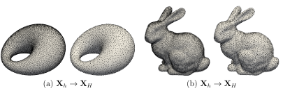
Figure B.2: Illustration of the WSE algorithm for generating a coarse level set XH of NH = Nh 4 points from a ne level set Xh of Nh points. Here Nh =14561 & NH =3640 for the cyclide (a) and Nh = 14634 & NH = 3658 for the Stanford Bunny (b) .

involving the interpolation Ih H and restriction IH h operators, and is de ned as follows:

LH =IH hLhIhH (b.16)

This latter operator, referred to as the Galerkin coarse grid operator, provides a simple means of coarsening Lh and has been shown to be robust for a large class of problems, especially those where a direct discretization on the coarse grid does not adequately represent the approximation on the ne grid [45, §7.7.4]. It also gives rise to a variational principle that is exploited in the analysis of algebraic multigrid (AMG) [45, §A.2.4] methods. While this latter result relies on the matrix being symmetric positive de ne, modi cations to this theory have also been developed for non-symmetric problems, which involve choosing the restriction operator di erently than the transpose of the interpolation operator [30]. We use the Galerkin approach for forming LH, as we have found that it approximates the ne grid operator on the coarser levels better than the direct discretization technique and it makes for a more robust solver/preconditioner. While Lh is not symmetric for our discretizations, we have nonetheless found that simply choosing IH h = (Ih H)T works well over a large array of test problems.

One disadvantage of the Galerkin approach is that LH has to be formed explicitly through sparse matrix-matrix multiplication, which is more computationally expensive in terms of time and memory than the direct discretization approach. Several researchers have developed methods to reduce this cost on parallel architectures (e.g.,[6, 4]), but we have not used these methods in our implementation. We simply construct LH as part of a set-up phase using a sparse matrix library. However, we do some minor alterations to improve the computational performance. These include reordering the rows and columns of Lh to decrease its bandwidth using the reverse Cuthill-McKee (RCM) algorithm prior to forming LH. This essentially leads to a reordering of the nodes Xh, which in turn leads to a reordering of the interpolation operator Ih
H. We also use RCM to reorder the rows and columns of LH after it is formed, which leads to a re-ordering of the nodes Xh and of the columns of Ih
H. We have found that these matrix reorderings not only reduce the wall-clock time of MGM, but also the number of iterations to reach convergence.

B.5.3 Smoother and coarse level solver

For the smoothing operator we use classical Gauss-Seidel (GS) method. One application of the smoother can be written as

uh uh +B 1 h (fh -Lhuh) (b.16)

where Bh is the lower triangular part (called forward GS) or upper triangular part (called backward GS) of Lh. In some cases we vary the version of the smoother for the pre- and post- smoothing operations (e.g., forward GS for pre-smooth and backward GS for the post-smooth). We denote the number of applications of the smoother for the pre- and post-phases of the cycle as 1 and 2, respectively. To solve for the defect on the coarse level, we use a direct solver based on a sparse LU factorization of LH (e.g., SuiteSparse or SuperLU).

B.5.4 Modi cations to the two-level cycle for the surface
Poisson problem

When(B.3) corresponds to the discretization of a surface Poisson problem (Lh = Dh), the system is singular and some modi cations to the two level cycle in Algorithm 2 are necessary. To understand the nature of the singularity, we can look at the continuous problem (B.1). As discussed in Section B.2.1, this problem has a solution if and only if the right hand side satis es the compatibility condition. Furthermore, the solution is only unique up to the addition of a constant. The degeneracy in the continuous problem manifests in the discrete problem as a one dimensional null space of Lh corresponding to constant vectors. The discrete analog of the consistency condition is that (B.3) has a solution if and only if fh is orthogonal to the left null vector of Lh (i.e., fh is in the range of Lh). Also, similar to the continuous case, any solution of (B.3) is only unique up to the addition of a constant vector.

The primary issue that arises with using multilevel methods (and other iterative methods) for these types of singular systems stems from the fact that, in practice, fh is rarely in the range of Lh. This can cause the iterations to fail to converge to a suitable approximation. Three standard approaches to bypass this issue include the following. First, one can project fh into the range of Lh. However, this requires computing the left null vector, which can be computationally expensive2.

It also requires modifying the coarse level solver to use the pseudoinverse (or some approximate inverse). A second approach is to impose that the solution is zero at one point. This xes the non-uniqueness issue and transforms the problem into solving a non-singular system of one dimension smaller. However, this can lead to a deterioration of the convergence of the multilevel method since the pointwise condition is not well approximated on coarser levels [49]. Additionally, the solution to this approach can be less accurate and less smooth than the projection approach [51]. The third approach is to enforce a global constraint on the solution, such as the discrete mean of uh is zero [45, §5.6.4].

This constraint can be enforced using a Lagrange multiplier, which transforms the linear system into the constrained system

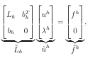
(b.18)

where bh is a row vector of length N with all of its components set to 1 (i.e., the summation operator), and h is the Lagrange multiplier. Provided bh is not orthogonal to the left null space of Lh (which is likely to be true because of the compatibility condition for the continuous problem), this constrained system will have a unique solution [45, Lemma 5.6.1]. Furthermore, if this condition holds, the solution will be the same (up to a constant) as the projection approach, since fh h bT h is then necessarily in the range of Lh. We use the third approach in the MGM method. Some modi cations to the two-level cycle are required to handle the constrained 2Note that Lh is not symmetric, so the constant vector is not necessarily the left null vector system(B.18). First, the transfer operator shave toal so trans fer the Lagrangemul tipler through the neand coar selevels and the Galerkin coarsegrid operator has to
include the transferred constraint.We follow the approach from[1] and modify these operators according to the following definitions:

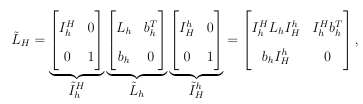
(b.19)

whereIh Hand I H h are the modified interpolation and restriction operators,respectively,
and LH is the modified Galerkin operator.The semodified transfer operators simply pass the Lagrange multiplier bet ween levels with out alteration. For the smoother of the constrained system(B.18),we use the approach discussed
in[45,§5.6.5],where only the solution u his smoothed and the constraintis left alone. We a gainuse GS for smoothing uh and one application of the modified smoother takes the form

uh uh+B 1 h (fh- Lhuh bh h),

where Bh is the same as(B.17). This smoother is equivalent too neiteration of the un damp edin exact Uzawa method with the Schur complement set equal to zero[7]. Finally,we use adirect solve to compute the defecte hand Lagrange multiplier H on the coarse level. This system takes the form LHeH=rH,whereeH= eH H
T andr His the restricted residual for the modified system: rH=IH h(fh Lhuh).When solving a Poisson problem,we use the modifications described abovein Algorithm2.

Algorithm 3: MGM preprocessing phase
1 Input: Fine level nodes X1 and operator L1; minimum number of coarse level points Nmin;

2 Re-order rows and columns of L1 using RCM;
3 Re-order X1 according to the RCM ordering;
4 Compute number of levels: p = log(N1Nmin) log(4) +1;
5 for j = 1 p 1do
6 Generate coarse point cloud Xj+1 with Nj+1 = N1 4j points ;
7 Generate interpolation operator Ij j+1 from Xj+1 to Xj;
8 Set the restriction operator to Ijj+1 =(Ij j+1)T;
9 Generate Galerkin coarse level operator Lj+1 = Ij j+1LjIj+1
10 Re-order rows and columns of Lj+1 using RCM;
11 Re-order rows of Ij j+1 and columns of Ijj+1jj according to the RCM ordering;
12 end
13 Compute sparse LU decomposition of Lp;

B.5.5 Multilevel extension

The multilevel extension of the two-level cycle can be obtained by applying it recursively until a sufficiently coarse level is reached to make a direct solver practical. To simplify the notation in describing the multilevel cycle, we replace the hH super script/subscript notation with a number corresponding to the level, with j = 1 being the nest level. For example, for the jth level, Xj denotes the point cloud, Nj denotes its size, Lj denotes the operator, rj denotes the residual, and Ij+1 j to level j + 1. is the restriction Before the multilevel cycle begins, we compute all the coarse point clouds, trans fer operators, and Galerkin coarse level operators in a preprocessing step, which is outlined in Algorithm 3. The number of levels, p, depends on the number of ne level nodes and minimum number of nodes on the coarsest level, Nmin, and is determined on line 4 of this algorithm. This guarantees that the number of nodes on the coarsest
level satis es Nmin Np < 4Nmin. We note that when using WSE to generate the coarse point cloud Xj on line 6 of the preprocessing algorithm, we use the ner point cloud Xj+1, rather than the nest node X1. This reduces the cost in performing this step.

The multilevel cycle is outlined in Algorithm 4 in non-recursive form. This algorithm is what we call the MGM method and corresponds to a traditional V-cycle in multigrid methods, which is typically denoted V( 1 2) corresponding to the number of pre-/post smoothing operations. Other cycling methods can also be used (e.g., F or W-cycle [45, §2.4]), but we limit our focus to the V-cycle. While this algorithm is described for a shifted Poisson problem, it can be easily modi ed for solving a Poisson problem following the modi cations discussed in Section B.5.4.

Algorithm 4: MGM V( 1 2)-cycle

1 Input: Right hand side f1; Initial guess u1; Number levels p; {Lj} p 1 j=1;

{Ijj+1} p 1 j=1; {Ijj+1} p 1 j=1;
2 RCM re-orderings; Sparse LU factorization of Lp;
3 Re-order f1 and u1 according to RCM re-ordering of L1;

4 Presmooth initial guess: u1 presmooth(L1 u1 f1 1);
5 Compute/restrict residual: r1 = I2 1(f1 L1uh)

7 Presmooth defect: ej = presmooth(Lj 0rj 1) ;

8 Compute/restrict residual: rj+1 = Ij+1 j (rj Ljej) ;

9 end

10 Compute defect: Solve Lpep = rp using sparse LU decomposition of Lp ;
11 for j = p 1 2do

12 Interpolate/correct defect: ej ej +Ij j+1ej+1;
13 Post smooth defect: ej posts mooth(Lj ej rj 2);
14 end

15 Interpolate defect/correct approximation: u1 u1 +I1 2e2;
16 Post smooth approximation: u1 posts mooth(L1 u1 f1 2);
17 Undo re-ordering of u1 from RCM of re-ordering of L1;

B.5.6 Preconditioner for Krylov subspace methods

The MGM method has the bene t of being relatively straightforward to implement. However, as shown in the numerical experiments in the next section, it may converge slowly when using it as a standalone solver, especially for higher order discretizations of the LBO on more irregular point clouds. A common approach to bypassing these issues for standard geometric and algebraic multigrid methods is to combine them with a Krylov subspace method (e.g., [45, §7.8] or [33, 18]). In this case, multi grid is viewed as preconditioner for the Krylov method. We also take this approach with MGM, using it a preconditioner for two Krylov methods: generalized minimum residual (GMRES) and bi-conjugate gradient stabilized (BiCGSTAB) [37]. This com bination appears to result in an e cient and robust method for solving the discretized surface Poisson and shifted Poisson equations on quite complicated surface.

B.6 Numerical Results

In this section, we analyze the MGM method as a solver and preconditioner for the Poisson and shifted Poisson problem on two surfaces: the unit sphere and the cyclide. The latter is shown in Figure B.2 and the implicit equation describing the surface is given in [26]. We test the method on both RBF-FD and GFD discretizations using the parameters given in the rst part of Table B.1. In all the tests, we are interested in how the method scales to higher order discretizations, and thus give results for polynomial degrees = 3, 5, and 7, which correspond to approximately second, fourth, and sixth order accuracy, respectively [41, 43]. For the sphere tests, we generate the point clouds from the vertices of icosahedral node sets, which are used extensively in numerical weather prediction [? ]. For the cyclide, we use point

Variable Description Value(s)
Parameters for the discretization the LBO
l Poly. degree for discretizing the LBO with RBF-FD or GFD 3, 5, or 7

k Order of the PHS kernel for discretizing the LBO with RBF-FD l

a Weighting parameter for the Gaussian kernel in GFD 4 or 5 4 or 5

n Stencil size for discretizing the LBO with RBF-FD or GFD ( +1)( +2)

Parameters for MGM

N min Minimum number of nodes on the coarsest level 250

Bh Pre- and post-smoother (see (B.17)) Forward GS

v1 v2 Numberof applications of the pre- and post-smoother 1

m Stencil size of the interpolation/restriction operators 2

Table B.1: Description of parameters and their values used in the numerical results.

clouds produced from Poisson disk sampling of the surface. This latter approach results in much more unstructured point clouds than the sphere case (see Figure B.2 for an illustration). Unless otherwise speci ed, the parameters of the MGM method are set according to those given in the second part of Table B.1. We tested the method with di erent combinations of these parameters and found that the ones listed in the table generally gave the best results in terms of iteration count and wall-clock time. Additionally, when using MGM with Krylov methods, we use it as a right preconditioner, which is generally recommended [18]. Finally, all the MGM results presented were obtained from a MATLAB implementation of the method, with a MEX interface to the WSE
method, which is implemented in C++. In the rst several experiments, we compare MGM to AMG, as implemented in the Python package PyAMG [32]. In addition to being very popular blackbox solvers and preconditioners for a wide range of problems, AMG methods have been used previously for solving linear systems associated with meshfree discretizations of elliptic PDEs in the plane [38] and on surfaces [20]. We use the smoothed aggregation version of AMG, as we found it performed better than classical AMG. Additionally, we use one application of symmetric GS as the pre- and post-smoother, a V-cycle for the multilevel cycle, and sparse LU for the coarse level solver. We experimented with other combinations of parameters and again found these generally gave the best results in terms of iteration count and wall-clock time. Additionally, when using PyAMG with GMRES, we use it as a right preconditioner (with the fgmres option), while for BiCGSTAB we use it as a left preconditioner (as this is the only option).

Finally, in the comparisons with AMG, we focus on the shifted Poisson problem as PyAMG does not o er a specialized way to deal with the constrained system (B.18).

B.6.1 Standalone solver vs. preconditioner

In the rst set of tests, we compare MGM and PyAMG both as standalone solvers and preconditioners. For the latter approaches we refer to these solvers as MGM GMRES, MGMBiCGSTAB, PyAMG GMRES, and PyAMG BiCGSTAB, to indicate the type of Krylov method employed. We use these solvers on the shifted Poisson problem on the unit sphere and cyclide with Nh=2,621,422 and Nh=2,097,152 nodes, respectively. For the BiCGSTAB results, we count the number of applications of the preconditioner as the iterations since each step of this method applies the preconditioner twice, whereas GMRES applies it once.

Figure B.3 displays the results in terms of relative residual vs. iteration count for RBF-FD, while Figure B.4 displays the results for GFD. For the RBF-FD results, we see that the methods using MGM converge more rapidly than the methods based on PyAMG for both surfaces. For the sphere, MGM works very well as a standalone solver and preconditioner even as increases, but for the cyclide the convergence rates of MGM as a standalone solver decrease considerably. This may be due to the more irregular nature of the cyclide point cloud. We note, however, that the preconditioned versions of MGM only have a very mild decrease in convergence rates for the cyclide.

The gures also show that the methods using PyAMG do not converge as rapidly as the corresponding MGM methods, with the fastest converging PyAMG method taking more than double the number of iterations as the fastest MGM method when =3andtriple when = 5and7. Weseesimilar patterns in the GFD results, but the methods based on both MGM and PyAMG generally converge faster in this case and the gap between the fastest converging MGM and PyAMG methods is not as wide. Finally, we note that MGM BiCGSTAB seems to converge at a very similar rate to MGMGMRES,whereas this does not hold for PyAMG. This is a promising result for large systems since the storage requirements of BiCGSTAB are xed, whereas they grow with the size of the Krylov subspace for GMRES [18].

These experiments also indicate that, while MGM can be an e ective standalone solver for small (lower order discretizations), it is more robust for larger (higher order discretizations) and when used as a preconditioner. This also seems to be the case when applying it to di erent surfaces and point clouds based on regular nodes (like the sphere) and irregular nodes (like the cyclide). From the PyAMG results, it is clear that it should be used as a preconditioner to get the most robust results, which is generally the case for AMG methods applied to nonsymmetric systems [18].

Sphere

PyAMG MGM

N L=3 L =5 L=7 L =3 L=5 L=7
10242 30 (38) 39 (56) 46 (70) 18 (19) 18 (18) 18 (20)
40962 35 (42) 43 (54) 53 (78) 19 (19) 19 (20) 19 (20)
163842 40 (50) 49 (64) 59 (84) 19 (21) 19 (20) 19 (20)
655362 45 (62) 55 (80) 68 (90) 20 (20) 20 (20) 20 (21)
2621442 52 (66) 64 (102) 75 (94) 20 (21) 20 (22) 20 (22)

Cyclide

PyAMG MGM

N L =3 L=5 L=7 L=3 L=5 L =7

8192 25 (30) 34 (48) 42 (62) 17 (19) 19 (20) 20 (22)
32768 32 (40) 39 (48) 46 (64) 19 (20) 22 (22) 24 (26)
131072 35 (46) 45 (66) 54 (74) 20 (21) 23 (26) 28 (31)
524288 41 (50) 49 (68) 60 (78) 21 (22) 25 (27) 30 (39)
2097152 45 (54) 56 (78) 65 (90) 20 (21) 24 (25) 27 (29)

Table B.2: Comparison of the number of PyAMG and MGM preconditioned GMRES/BiCGSTABiterations required to reach a relative residual tolerance of 10 12 for solving the shifted Poisson problem with RBF-FD discretizations. The numbers not in parenthesis are for GMRES, while the numbers in parenthesis are for BiCGSTAB.

B.6.2 Scaling with problem size

In the next set of tests, we examine how both the MGM and PyAMG methods scale as the size of the point clouds Nh increases. We focus on the preconditioned versions of these methods and test them again on the sphere and cyclide. Tables B.2 and B.3 display the results for the RBF-FD and GFD methods, respectively, in terms of number of iterations required to reach a relative residual of 10 12. We see from these tables that the preconditioned MGM methods appear to scale much better than the PyAMG methods, both in terms of Nh and . For RBF-FD discretizations, the increase in the iteration count for MGM is more mild with increasing than for GFD. However, in all cases but = 7 on the sphere, the iteration count is lower for the GFD discretizations; we examine this further in Section B.6.4.

Sphere

PyAMG MGM

N L=3 L=5 L=7 L=3 L=5 L =7

10242 15 (18) 20 (26) 26 (34) 10 (10) 14 (14) 20 (21)
40962 17 (20) 23 (26) 30 (42) 10 (11) 15 (16) 23 (25)
163842 20 (22) 27 (36) 34 (42) 11 (12) 15 (17) 26 (29)
655362 23 (26) 30 (42) 39 (48) 12 (13) 16 (17) 27 (28)
2621442 27 (30) 35 (46) 43 (60) 13 (15) 16 (17) 27 (29)

Cyclide

PyAMG MGM

N L=3 L=5 L= 7 L =3 L=5 L=7
8192 13 (16) 17 (20) 23 (28) 10 (11) 14 (14) 18 (19)
32768 16 (20) 21 (24) 26 (30) 12 (12) 17 (18) 24 (26)
131072 19 (24) 24 (32) 30 (36) 12 (13) 18 (21) 25 (27)
524288 22 (26) 27 (34) 34 (40) 13 (14) 18 (18) 26 (29)
2097152 25 (30) 32 (40) 39 (50) 14 (14) 17 (18) 24 (26)

Table B.3: Same as Table B.2, but for GFD discretizations. For these results, we set = 4 for all Nh, but the largest, where we set = 5.

In Figure B.5 we display the wall-clock times for the results in Tables B.2 and B.3 for GMRES PyAMG and MGM. These results were run on a Linux Workstation with Intel i9-9900X 3.5 GHz processor (with no explicit parallelization) and do not include the set-up times. We see from Figure B.5 that MGM has a lower wall-clock time than PyAMG for all but the rst Nh in the case of the sphere. Furthermore, for the largest Nh, MGM is between 3 and 5 times faster. Additionally, the dotted line in these scaling plots marks perfect linear scaling and we see that the results for both methods have a very similar slope to this line. Finally, we note that the timing results for BiCGSTAB follow a similar trend to GMRES, so we omitted displaying the results. However, the gap between the MGM and PyAMG timings were larger in this case.

B.6.3 Spectrum analysis

The previous two sections showed the preconditioned MGM methods outperforming the PyAMG methods. To better understand these results, we investigate the spectrum (eigenvalues) of the preconditioned matrices from both methods. Letting Mh denote the matrix representation for applying one V-cycle of either MGM or PyAMG, we can write the (right) preconditioned system as LhMhzh = fh, where zh = (Mh) 1uh. The convergence behavior of Krylov methods can be understood by analyzing the spectrum LhMh. As discussed in, for example [34], the more clustered
this spectrum is to one, the faster the Krylov methods will converge. In Figure B.6 we display the complete spectrum of the preconditioned matrix LhMh of both MGM and PyAMG for the RBF-FD discretizations on the sphere and cyclide. Due to the cost of this eigenvalue computation, we were only able to compute the results for with Nh =10242 and 8192, respectively. We see from the gure that spectra for MGM are more clustered around one than PyAMG for both surfaces and increasing , which explains the better iteration counts in Table B.2. We omit the results for GFD, but note that the spectra were similar to RBF-FD, but were even more clustered near one.

B.6.4 Iteration vs. accuracy

In the nal set of tests we focus on solving the (discretized) Poisson problem with MGMGMRES and examine how the accuracy of the RBF-FD and GFD discretizations depend on the iteration count for increasing Nh and . We restrict our at tention to the sphere, for which it is easy to construct test problems with exact solutions based on spherical harmonics. For the test problem in the experiments, we use the Y4 5 spherical harmonic, which can be written in Cartesian coordinates as Y4 5(xy z) = z(x4 6x2y2+y4). We x the number of iterations of MGM GMRES for solving the discretized systems to 151015202530, and compute both the relative residual and relative errors (in the 2-norm) in the approximate solutions. Figure B.7 displays the results from these experiments. We see from the gure that in almost all cases the minimum error for either the RBF-FD and GFD is reached before the minimal residual is reached. Additionally, the results indicate that while the residuals for GFD converge faster than RBF-FD, the errors for a given Nh and are smaller for RBF-FD. So the cost per error for both methods is much more comparable than the previous experiments indicated and favor RBF-FD.

B.7 Applications

In this section we demonstrate the performance of MGM on three di erent applications involving complicated surfaces represented by relatively large point clouds; see Figure B.8. All these applications involve solving discrete (shifted) surface Poisson problems, for which we use the RBF-FD method to approximate the LBO and MGM GMRES to solve the resulting linear systems.

B.7.1 Surface harmonics

We rst consider approximating the rst several eigenvalues and eigenfunctions of the LBO on the Chinese Guardian Lion model. The eigenfunctions of the LBO or the surface harmonics have been used in various applications in data analysis. For example, Reuter et. al. [36] used the low frequency surface harmonics for shape segmentation and registration. The LBO eigenvalue problem is given as Mu = u. To approximate the solutions of this problem we use the RBF-FD method with = 5 to approximate the LBO and ARPACK[25] (accessed through the eigs function in MATLAB) to solve the discrete system for the rst several eigenpairs that are smallest in magnitude. ARPACK uses the Arnoldi method on the shifted inverse of a matrix to nd the eigenpairs closest to the shift , which, for the surface problem, requires a routine for repeatedly solving systems of the form (Lh Ih)vh = fh, for di erent fh. We use MGM GMRES to solve these linear systems with = 1 and set the tolerance to 10 10. Figure B.9
displays the rst 10 non-zero harmonics computed with this technique. The ARPACK routine used 49 linear system solves to determine the eigenpairs; the median number of MGM GMRESiterations required to solve these systems was only 15 and the max was 16.

B.7.2 Pattern formation

We next consider solving two coupled reaction-di usion (RD) equations on the Stan ford Bunny model. These types of equations arise, for example, in phenomenological models of color patterns in animal coats [31]. We consider the Gierer-Meinhardt two-species RD system [19] given as follows:

uby t =Du Mu+A Bu+ u2 by v(1 +Cu2) (B.20a)
vbyt =Dv Mv+u2- v (B.20b)

By altering the parameters A, B, C, Du, and Dv appropriately, this system can produce solutions that converge to spot or labyrinth patterns at steady-state [31]. For the bunny model, we set A = 008, B = 15, C = 045, Du = 5 10 5, and Dv = 10 3 to produce the labyrinth pattern. We use a random initial condition, where at each point in Xh the values of u and v are selected from a uniformly random distribution in the interval [01].

To approximate the solution of (B.20) we use the RBF-FD method with = 3 to approximate the LBO and apply the second-order accurate semi-implicit backward difference scheme (SBDF2) [3] as the time-stepping method that treats the diffusion implicitly and reactions explicitly. We set the time-step to t = 005. The temporal discretization results in two decoupled (discrete) screened Poisson problems that need to be solved at each time-step for which we use GMRES preconditioned with MGM.

For the GMRES method we set the tolerance on the relative residual to 10 8 and use the previous time-step as the initial guess. We set the nal integration to 300 time units, which resulted in a near steady-state pattern. Figure B.10 displays the results of the simulations. Included in the gure are the iterations required by the preconditioned GMRES method as a function of time. We see from the gure that the maximum iteration count is 6 for the u variable and 11 for the v variable, and decreases to 2 and 3, respectively as the solutions approach steady-state. The larger iteration count for the v variable is expected since the di usion coe cient is larger in
(B.20b).

B.7.3 Geodesic distance

Lastly, we consider the classic problem of approximating the geodesic distance from a given point on a surface to all other points. We use the heat method introduced by Crane et. al. [11] to solve this problem. This method transforms the non-linear geodesic distance problem, typically formulated in terms of the eikonal equation, into solving a pair of linear parabolic and elliptic problems. The heat method is comprised
of the three steps: 1. Solve ut = Mu, with u0 = (x), to some time t nal > 0

2. Compute the vector eld = Mu
3. Solve the Poisson problem M = M Mu

Here x denotes the target point on the surface M to compute the distance from, M denotes the surface gradient, M is the surface divergence, and denotes the Dirac delta function. As discussed in [11], the function approximates the geodesic distance and converges to the exact distance as t nal0.

We apply the heat method on the Armadillo model. We again use the RBF-FD method with = 3 to approximate the LBO in steps 1 and 3 above. To approximate the surface gradient and divergence, we also use the RBF-FD method formulated in the tangent plane similar to the method described in [43] for GFD. For these approximations, we use = 2, which result in a second-order approximation. We discretize the heat equation in the rst step with backward Euler in time with a time-step of t = 10 3 and set t nal = 3 t. To solve the linear systems associated with this implicit discretization and the system from the discretized Poisson equation in step 3, we use GMRES preconditioned with MGM, setting the tolerance to 10 8.

The results for a point x on the chest of the Armadillo are displayed in the rst to images of Figure B.11. The last image in this gure displays the iterations of the preconditioned GMRES method for solving the systems from the heat equation discretization for three time-steps and the Poisson system to determine . We see that the iteration count remains low for all these systems.

B.8 Concluding remarks

We have presented a new geometric multilevel method, MGM, for solving linear systems associated with discretizations of elliptic PDEs on point clouds. The method is entirely meshfree and uses the WSE algorithm for coarsening the point clouds, interpolation/restrictions operators based on polyharmonic spline RBFs, Galerkin coarsening of the operator, and standard smoothers. All of these choices make MGM particularly straightforward to implement. We numerically analyzed the method as a standalone solver and preconditioner on test problems for the sphere and cyclide discretized using RBF-FD and GFD methods, and found that it compares favorably to AMGmethods in terms of convergence rates and wall-clock time. When using MGM as a preconditioner, we also found that it scaled well as both the problem size and accuracy of the discretizations increased. Finally, we demonstrated that the method can be used in three challenging applications involving large systems of equations.

There are several extensions of MGM that we plan to pursue in the future. One is to test the method on other discretizations. MGM is agnostic to the underlying discretization and could be used even for (nodal) mesh-based discretizations. Here the nodal points of the mesh could be treated as a point cloud and WSE could be applied, or if there is a natural way to coarsen the mesh, then this could be used instead. A second idea we plan to pursue is extending MGM to domains with boundaries, which in principle should be straightforward. Finally, we plan to look into parallel implementations of the method to further improve the performance.

Acknowledgements

AMJ and GBWs work was partially supported by US NSF grants CCF-1717556 and DMS-1952674. VSs work was partially supported by US NSF grants CCF-1714844.

We bene tted from discussions with Drs. Cem Yuksel (on the WSE algorithm) and Hari Sundar (on multigrid methods), both from the University of Utah. The Stanford Bunny and Armadillo data were obtained from the Stanford University 3D Scanning Repository. The Chinese Guardian Lion data was obtained from the AIM@SHAPE
VISIONAIR Shape Repository.

REFERENCES

[1] Adams, Mark F. 2004. Algebraic multigrid methods for constrained linear systems with applications to contact problems in solid mechanics. Numerical Linear Algebra with Applications, 11, 141153.

[2] Alvarez, Diego, Gonzalez-Rodrguez, Pedro, and Kindelan, Manuel. 2021. A Local Radial Basis Function Method for the LaplaceBeltrami Operator. J. Sci. Comput., 86(3), 28.

[3] Ascher, Uri M., Ruuth, Steven J., and Wetton, Brian T. R. 1997. Implicit-Explicit Methods For Time-Dependent PDEs. SIAM J. Num. Anal, 32, 797823.

[4] Ballard, Grey, Siefert, Christopher, and Hu, Jonathan. 2016. Reducing Communication Costs for Sparse Matrix Multiplication within Algebraic Multigrid. SIAM J. Sci. Comput., 38(3), C203C231.

[6] Bell, Nathan, Dalton, Steven, and Olson, Luke N. 2012. Exposing Fine-Grained Parallelism in Algebraic Multigrid Methods. SIAM J. Sci. Comput., 34(4), C123 C152.

[7] Benzi, Michele, Golub, Gene H, and Liesen, Jorg. 2005. Numerical solution of saddle point problems. Acta Numerica, 14, 1137.

[8] Bertalmo, M., Cheng, L., Osher, S., and Sapiro, G. 2001. Variational problems and partial di erential equations on implicit surfaces. J. Comput. Phys., 174, 759780.

[9] Bridson, Robert. 2007. Fast Poisson Disk Sampling in Arbitrary Dimensions. In: ACM SIGGRAPH 2007 Sketches. SIGGRAPH 07. New York, NY, USA: ACM.

[10] Chen, Yujia, and Macdonald, Colin B. 2015. The closest point method and multigrid solvers for elliptic equations on surfaces. SIAM Journal on Scienti c Computing, 37(1), A134A155.

[11] Crane, Keenan, Weischedel, Clarisse, and Wardetzky, Max. 2013. Geodesics in heat: A new approach to computing distance based on heat ow. ACM Transactions on Graphics (TOG), 32(5), 111.

[12] Davydov, Oleg, and Schaback, Robert. 2019. Optimal stencils in Sobolev spaces. IMA J. Num. Analy., 39(1), 398422.

[13] Demanet, Laurent. 2006. Painless, highly accurate discretizations of the Laplacian on a smooth manifold. Technical report, Stanford University.

[14] Duchon, J. 1977. Splines minimizing rotation-invariant semi-norms in Sobolev space. Pages 85100 of: Schempp, W., and K., Zeller (eds), Constructive Theory of Functions of Several Variables. Lecture Notes in Mathematics (vol 571). Berlin: Springer.

[15] Dziuk, G. 1988. Finite elements for the Beltrami operator on arbitrary surfaces. In: Hildebrandt, S., and Leis, R. (eds), Partial Di erential Equations and Calculus of Variations. Lecture Notes in Mathematics, vol. 1357. Berlin: Springer.

[16] Dziuk, Gerhard, and Elliott, Charles M. 2013. Finite element methods for surface PDEs. Acta Numerica, 22, 289396.

[17] Fuselier, E, and Wright, G B. 2012. Scattered Data Interpolation on Embedded Submanifolds with Restricted Positive De nite Kernels: Sobolev Error Estimates. SIAM J. Numer. Anal., 50(3), 17531776.

[18] Ghai, Aditi, Lu, Cao, and Jiao, Xiangmin. 2018. A comparison of preconditioned Krylov subspace methods for large-scale nonsymmetric linear systems. Numerical Linear Algebra with Applications, 26(10).

[19] Gierer, Alfred, and Meinhardt, Hans. 1972. A theory of biological pattern for mation. Kybernetik, 12(1), 3039.

[20] Gross, B. J., Trask, N., Kuberry, P., and Atzberger, P. J. 2020. Meshfree methods on manifolds for hydrodynamic ows on curved surfaces: A Generalized Moving Least-Squares (GMLS) approach. J. Comput. Phys., 409, 109340.

[21] Gunderman, David, Flyer, Natasha, and Fornberg, Bengt. 2020. Transport schemes in spherical geometries using spline-based RBF-FD with polynomials. J. Comput. Phys., 408, 109256.

[22] Katz, Aaron, and Jameson, Antony. 2009. Multicloud: Multigrid convergence with a meshless operator. J. Comput. Phys., 228(14), 52375250.

[23] Klasing, K., Altho , D., Wollherr, D., and Buss, M. 2009. Comparison of surface normal estimation methods for range sensing applications. Pages 32063211 of: IEEE International Conference on Robotics and Automation.

[24] Landsberg, Christoph, and Voigt, Axel. 2010. A multigrid nite element method for reaction-di usion systems on surfaces. Computing and visualization in science, 13(4), 177185.

[25] Lehoucq, Richard B, Sorensen, Danny C, and Yang, Chao. 1998. ARPACK users guide: solution of large-scale eigenvalue problems with implicitly restarted Arnoldi methods. Philadelphia, PA, USA: SIAM.

[26] Lehto, E, Shankar, V, and Wright, G. B. 2017. A radial basis function (RBF) compact nite di erence (FD) scheme for reaction-di usion equations on surfaces. SIAM J. Sci. Comput., 39, A219A2151.

[27] Liang, Jian, and Zhao, Hongkai. 2013. Solving Partial Di erential Equations on Point Clouds. SIAM J. Sci. Comput., 35(3), A1461A1486.

[28] Liu, Jinghui, Totz, Jan F., Miller, Pearson W., Hastewell, Alasdair D., Chao, Yu-Chen, Dunkel, Jorn, and Fakhri, Nikta. 2021. Topological braiding and virtual particles on the cell membrane. Proc. Natl. Acad. Sci. U.S.A., 118(34).

[29] MacDonald, C. B., and Ruuth, S. J. 2009. The implicit closest point method for the numerical solution of partial di erential equations on surfaces. SIAM J. Sci. Comput., 31, 43304350.

[30] Manteu el, Tom, and Southworth, Ben S. 2019. Convergence in Norm of Non symmetric Algebraic Multigrid. SIAM Journal on Scienti c Computing, 41(5), S269S296.

[31] Miyazawa, Seita, Okamoto, Michitoshi, and Kondo, Shigeru. 2010. Blending of animal colour patterns by hybridization. Nature communications, 1(1), 16.

[32] Olson, L. N., and Schroder, J. B. 2018. PyAMG: Algebraic Multigrid Solvers in Python v4.0. Release 4.0.

[33] Oosterlee, C. W., Wienands, R., Washio, T., and Gaspar, F. J. 2000. The acceleration of multigrid convergence by recombination techniques. Pages 3443 of: Multigrid methods, VI (Gent, 1999). Lect. Notes Comput. Sci. Eng., vol. 14. Berlin: Springer.

[34] Oosterlee, Cornelis W, and Washio, Takumi. 1998. An evaluation of parallel multigrid as a solver and a preconditioner for singularly perturbed problems. SIAM Journal on Scienti c Computing, 19(1), 87110.

[35] Piret, Cecile, and Dunn, Jarrett. 2016. Fast RBF OGr for solving PDEs on arbitrary surfaces. AIP Conference Proceedings, 1776(1), 070005.

[36] Reuter, Martin, Biasotti, Silvia, Giorgi, Daniela, Patane, Giuseppe, and Spagnuolo, Michela. 2009. Discrete LaplaceBeltrami operators for shape analysis and segmentation. Comput. Graph., 33(3), 381390.

[37] Saad, Y. 2003. Iterative Methods for Sparse Linear Systems. Philadelphia: SIAM.

[38] Seibold, Benjamin. 2010. Performance of algebraic multigrid methods for non symmetric matrices arising in particle methods. Numerical Linear Algebra with Applications, 17(2-3), 433451.

[39] Shankar, Varun, Wright, Grady B., Kirby, Robert M., and Fogelson, Aaron L. 2014. A Radial Basis Function (RBF)-Finite Di erence (FD) Method for Diffusion and Reaction-Di usion Equations on Surfaces. J. Sci. Comput., 63(3), 745 768.

[40] Shankar, Varun, Narayan, Akil, and Kirby, Robert M. 2018. RBF-LOI: Augmenting Radial Basis Functions (RBFs) with Least Orthogonal Interpolation (LOI) for solving PDEs on surfaces. J. Comput. Phys., 373, 722735.

[41] Shaw, Sage. 2019. Radial Basis Function Finite Di erence Approximations of the Laplace-Beltrami Operator. M.Phil. thesis, Boise State University, USA. 1587.

[42] Stoop, Norbert, Lagrange, Romain, Terwagne, Denis, Reis, Pedro M, and Dunkel, Jorn. 2015. Curvature-induced symmetry breaking determines elastic surface patterns. Nature materials, 14(3), 337342.

[43] Suchde, Pratik, and Kuhnert, Jorg. 2019. A meshfree generalized nite di erence method for surface PDEs. Comp. Math. Appl., 78(8), 27892805.

[44] Trask, Nathaniel, and Kuberry, Paul. 2020. Compatible meshfree discretization of surface PDEs. Computational Particle Mechanics, 7, 271277.

[45] Trottenberg, Ulrich, Oosterlee, Cornelis W., and Schuller, Anton. 2001. Multi grid. Texts in Applied Mathematics., vol. 33. Academic Press.

[46] Turk, Greg. 1991. Generating textures on arbitrary surfaces using reaction diffusion. Comput. Graph., 25(4), 289298.

[47] Wendland, Holger. 2005. Scattered data approximation. Cambridge Monogr. Appl. Comput. Math., vol. 17. Cambridge: Cambridge University Press.

[48] Wendland, Holger, and Kunemund, Jens. 2020. Solving partial di erential equations on (evolving) surfaces with radial basis functions. Advances in Computational Mathematics, 46, 64.

[49] Wesseling, P. 1992. An Introduction to Multigrid Methods. New York: John Wiley & Sons.

[50] Williamson, David L. 2007. The Evolution of Dynamical Cores for Global At mospheric Models. J. Meteorol. Soc. Jpn., 85B, 241269.

[51] Yoon, Myoungho, Yoon, Gangjoon, and Min, Chohong. 2016. On Solving the Singular System Arisen from Poisson Equation with Neumann Boundary Condition. J. Sci. Comput., 69, 391405.

[52] Yuksel, Cem. 2015. Sample Elimination for Generating Poisson Disk Sample Sets. Computer Graphics Forum (Proceedings of EUROGRAPHICS 2015), 34(2), 25 32.

[53] Yuksel, Cem. 2021. cyCodeBase.

[54] Zamolo, Riccardo, Nobile, Enrico, and Sarler, Bozidar. 2019. Novel multilevel techniques for convergence acceleration in the solution of systems of equations arising from RBF-FD meshless discretizations. J. Comput. Phys., 392, 311 334.

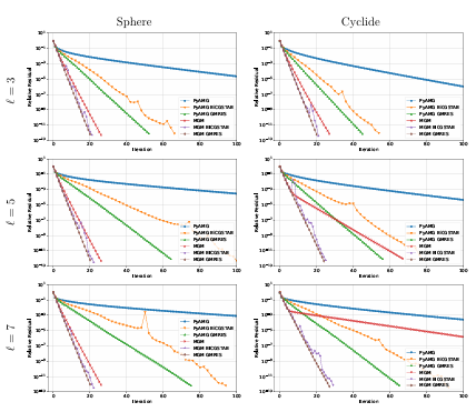
FigureB.3:ConvergenceresultsforMGMandPyAMGbasedsolversfor
RBF-FDdiscretizationsof ashiftedPoissonproblemwithrandomright
handside. Thesphereresultsare forNh=2621442,while forthecyclide
Nh=2097152.

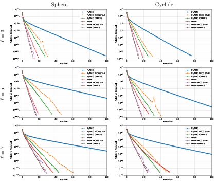
FigureB.4:SameasFigureB.3,butforGFDdiscretizationsoftheshifted
surfacePoissonproblem.

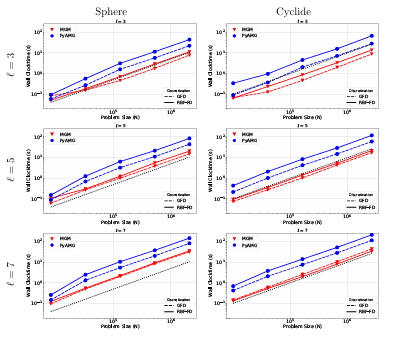
FigureB.5:Wall clock time (inseconds) for Py AMGGMRE Sand MGM GMREStoconvergetoarelativeresidualof 10 12 problem size (Nn) in creases forRBF-FD(solid line) andGFD(dashed line)discretizations. The black dotted line marks line ars caling , O(Nh), for reference.

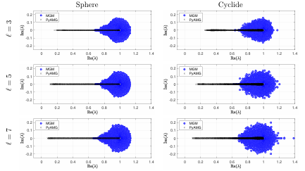
FigureB.6: ThespectraofthepreconditionedmatrixforshiftedPoisson
problemdiscretizedwithRBF-FD.

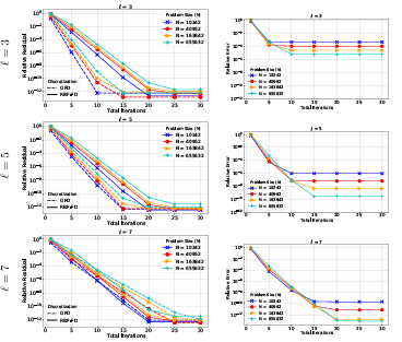
FigureB.7:Relativeresiduals(left)andrelative2 norm errors (right) for solving a Poisson problem on the sphere with MGMGMRES. Solidlines corres pond toRBF-FD discretizations,whiledashedlinescorrespondto GFD.

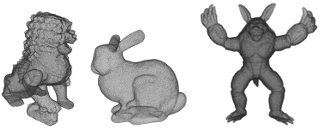
FigureB.8: Pointclouds for the surfaces considere din the applications: Chinese Guardian Lion (Nh=436605), Stan ford Bunny(Nh=291804),and Armadillo(Nh=872773).

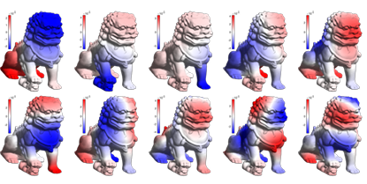
FigureB.9: Left: pseudocolormapof the rst10non-zerosurfacehar
monicsoftheChineseGuardianLionmodel.

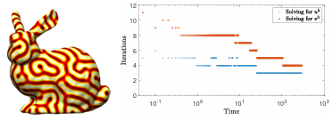
FigureB.10: Left: pseudocolormapof theuvariable in the numerical solution of (B.20) on the Stanford Bunny model;the colorstransitionfrom white to yellow tored to black ,withwhitecorrespondingtou=0and black to u=1. Right: iterationcountofMGMGMRESforsolvingthe
linear system sassociated withu and v variable satea ch time-stepinthe semi-implicitscheme for(B.20).

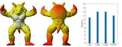
Figure B.11: Left: pseudocolor map of the approximate geodesic distance from the solid circle on the chest of the Armadillo model (viewed from the front and backside) computed with the heat method. Solid black lines mark the contours of the distance eld and the colors transition from white to yellow to red with increasing distance from the solid circle. Right: iteration count of GMRES preconditioned with MGM for solving the linear systems associated with the heat method.

In this article:

Click to comment

MESHFREE METHODS FOR PDES ON SURFACES

BOISE STATE UNIVERSITY GRADUATE COLLEGE

DEFENSE COMMITTEE AND FINAL READING APPROVALS

DEDICATION

ACKNOWLEDGMENT

Advisors and Collaborators

TABLEOFCONTENTS

LIST OF FIGURES

LIST OF FIGURES

CHAPTER 1:

INTRODUCTION

1.1 Overview

PI.

PII.

SI.

SII.

1.2 Mathematical modeling

1.3 Surface partial differential equations

1.4 Global meshfree interpolation and approximation

1.4.1 Radial basis functions

1.4.2 Polynomial moving least squares (MLS)

1.5 Localized meshfree methods

1.5.1 Stencils and nearest neighbor searches

1.5.2 RBF-FD

1.5.3 GMLS/GFD

1.6 Node generation

1.7 Contributions of this dissertation

1.7.1 Contributions of PI

Motivation

Overview

1.7.2 Contributions of PII

Motivation

Overview

1.7.3 Contributions of PI and PII

1.8 Future work

REFERENCES

CHAPTER 2:

A COMPARISON OF GENERALIZED MOVING LEAST SQUARES AND RADIAL BASIS FUNCTION FINITE DIFFERENCE METHODS FOR APPROXIMATING SURFACE DERIVATIVES

A.1 Abstract

A.2 Introduction

A.3.1 Stencils

A.3.2 Surface differential operators in local coordinates

A.4 GMLS using local coordinates

A.4.1 Approximating the metric terms

A.4.2 Approximating SDOs

A.4.3 Choosing the stencils and weight kernel

A.4.4 Approximating the tangent space

A.5 RBF-FD using the tangent plane

A.5.1 Tangent plane method

A.5.2 Approximating the SDOs

A.5.3 Choosing the stencils and PHS order

A.5.4 Approximating the tangent space

A.6 Theoretical comparison of GMLS and

RBF-FD

A.7 Numerical comparison of GMLS and RBF-FD

Table A.1: Sizes of the node sets used in the numerical experiments.

A.7.1 Convergence comparison: Sphere

A.7.2 Convergence comparison: Torus

A.7.3 E ciency comparison

A.8 Concluding remarks

Acknowledgements

REFERENCES

APPENDIX B: PAPER 2: MGM: A MESHFREE GEOMETRIC MULTILEVEL METHOD FOR LINEAR SYSTEMS ARISING FROM ELLIPTIC EQUATIONS ON POINT CLOUD SURFACES

B.1 Abstract

B.2 Introduction

B.3 Localized meshfree discretizations

B.3.1 Tangent plane method

B.3.2 PHS-based RBF-FD with polynomials

B.3.3 GFD

B.4 Multilevel transfer operators using RBFs

Algorithm 2: Two-Level Cycle

B.5 Meshfree geometric multilevel (MGM) method

B.5.1 Node coarsening

B.5.2 Coarse level operator

B.5.3 Smoother and coarse level solver

B.5.4 Modi cations to the two-level cycle for the surface Poisson problem

B.5.5 Multilevel extension

Algorithm 4: MGM V( 1 2)-cycle

B.5.6 Preconditioner for Krylov subspace methods

B.6 Numerical Results

A COMPARISON OF GENERALIZED MOVING
LEAST SQUARES AND RADIAL BASIS
FUNCTION FINITE DIFFERENCE METHODS
FOR APPROXIMATING SURFACE
DERIVATIVES

A.7 Numerical comparison of GMLS and
RBF-FD

APPENDIX B:
PAPER 2: MGM: A MESHFREE GEOMETRIC
MULTILEVEL METHOD FOR LINEAR
SYSTEMS ARISING FROM ELLIPTIC
EQUATIONS ON POINT CLOUD SURFACES

B.5 Meshfree geometric multilevel (MGM)
method

B.5.4 Modi cations to the two-level cycle for the surface
Poisson problem

Leave a Reply
Cancel reply